Paper I — Q8
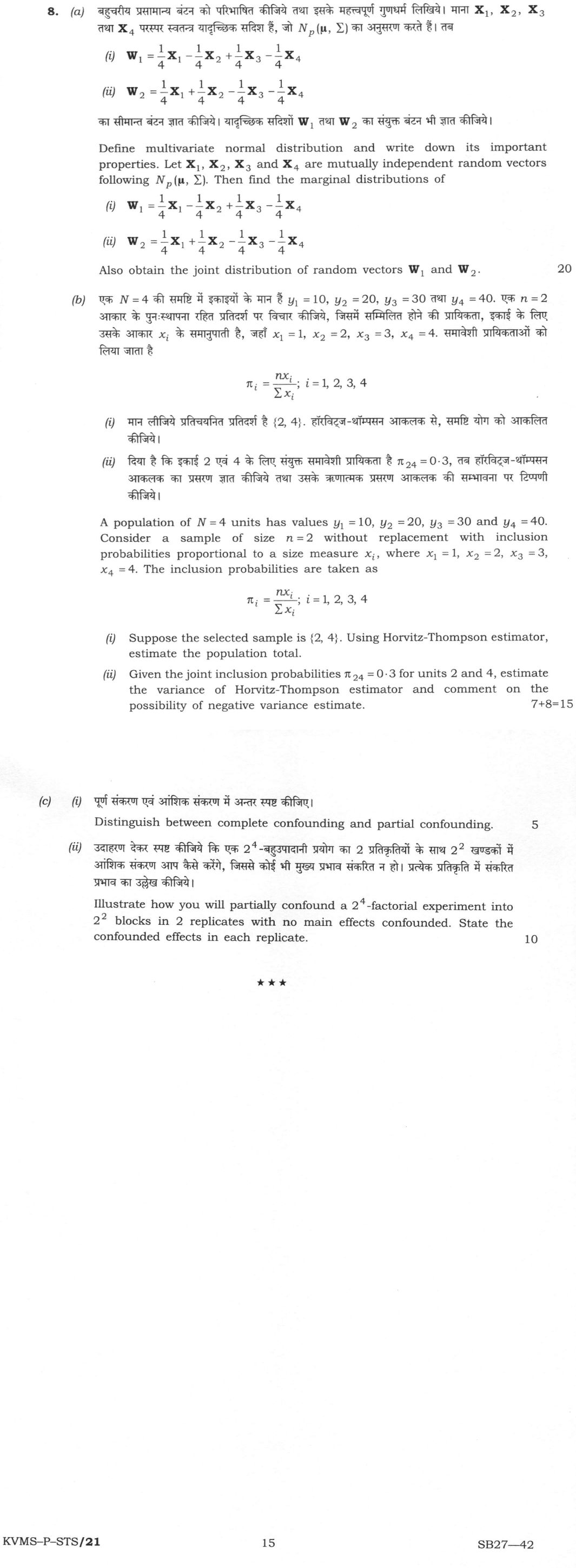
(a) Define multivariate normal distribution and write down its important properties. Let X₁, X₂, X₃ and X₄ are mutually…
Define multivariate normal distribution and write down its important properties. Let X₁, X₂, X₃ and X₄ are mutually independent random vectors following N_p(μ, Σ). Then find the marginal distributions of
W₁ = 1/4 X₁ − 1/4 X₂ + 1/4 X₃ − 1/4 X₄
W₂ = 1/4 X₁ + 1/4 X₂ − 1/4 X₃ − 1/4 X₄
Also obtain the joint distribution of random vectors W₁ and W₂. 20 marks
A population of N = 4 units has values y₁ = 10, y₂ = 20, y₃ = 30 and y₄ = 40. Consider a sample of size n = 2 without replacement with inclusion probabilities proportional to a size measure x_i, where x₁ = 1, x₂ = 2, x₃ = 3, x₄ = 4. The inclusion probabilities are taken as
π_i = nx_i / Σx_i ; i = 1, 2, 3, 4
Suppose the selected sample is {2, 4}. Using Horvitz-Thompson estimator, estimate the population total.
Given the joint inclusion probabilities π₂₄ = 0·3 for units 2 and 4, estimate the variance of Horvitz-Thompson estimator and comment on the possibility of negative variance estimate. 15 marks
Distinguish between complete confounding and partial confounding. 5 marks
Illustrate how you will partially confound a 2^4-factorial experiment into 2^2 blocks in 2 replicates with no main effects confounded. State the confounded effects in each replicate. 10 marks
हिंदी में प्रश्न पढ़ें
बहुचरीय प्रसामान्य बंटन को परिभाषित कीजिये तथा इसके महत्त्वपूर्ण गुणधर्म लिखिये। माना X₁, X₂, X₃ तथा X₄ परस्पर स्वतन्त्र यादृच्छिक सदिश हैं, जो N_p(μ, Σ) का अनुसरण करते हैं। तब
W₁ = 1/4 X₁ − 1/4 X₂ + 1/4 X₃ − 1/4 X₄
W₂ = 1/4 X₁ + 1/4 X₂ − 1/4 X₃ − 1/4 X₄
का सीमान्त बंटन ज्ञात कीजिये। यादृच्छिक सदिशों W₁ तथा W₂ का संयुक्त बंटन भी ज्ञात कीजिये। (20 अंक)
एक N = 4 की समष्टि में इकाइयों के मान हैं y₁ = 10, y₂ = 20, y₃ = 30 तथा y₄ = 40. एक n = 2 आकार के पुनःस्थापना रहित प्रतिदर्श पर विचार कीजिये, जिसमें सम्मिलित होने की प्रायिकता, इकाई के लिए उसके आकार x_i के समानुपाती है, जहाँ x₁ = 1, x₂ = 2, x₃ = 3, x₄ = 4. समावेशी प्रायिकताओं को लिया जाता है
π_i = nx_i / Σx_i ; i = 1, 2, 3, 4
मान लीजिये प्रतिचयनित प्रतिदर्श है {2, 4}. हॉरविट्ज़-थॉम्पसन आकलक से, समष्टि योग को आकलित कीजिये।
दिया है कि इकाई 2 एवं 4 के लिए संयुक्त समावेशी प्रायिकता है π₂₄ = 0·3, तब हॉरविट्ज़-थॉम्पसन आकलक का प्रसरण ज्ञात कीजिये तथा उसके ऋणात्मक प्रसरण आकलक की सम्भावना पर टिप्पणी कीजिये। (15 अंक)
पूर्ण संकरण एवं आंशिक संकरण में अन्तर स्पष्ट कीजिए। (5 अंक)
उदाहरण देकर स्पष्ट कीजिये कि एक 2^4-बहुउपादानी प्रयोग का 2 प्रतिकृतियों के साथ 2^2 खण्डकों में आंशिक संकरण आप कैसे करेंगे, जिससे कोई भी मुख्य प्रभाव संकरित न हो। प्रत्येक प्रतिकृति में संकरित प्रभाव का उल्लेख कीजिये। (10 अंक)
Model answer
Drafted with AI by UPSC Answer Check against this question's marking rubric, to the expected length. UPSC does not publish answers for Mains — this is one way to score well, not an official key. How we build rubrics and answers.
(a) Multivariate normal distribution; distributions of W₁ and W₂
Definition: a p-vector X follows Nₚ(μ, Σ) if every linear combination a′X is univariate normal N(a′μ, a′Σa); equivalently its characteristic function is φ_X(t) = expit′μ − ½t′Σt. When Σ is positive definite the density is f(x) = (2π)^(−p/2) |Σ|^(−1/2) exp−½(x − μ)′Σ⁻¹(x − μ).
Important properties: (i) AX + b ~ N_q(Aμ + b, AΣA′) for any q × p matrix A; (ii) all marginal distributions are normal, and conditional distributions are normal with mean linear in the conditioning variables and constant dispersion; (iii) for jointly normal vectors, zero covariance implies independence; (iv) (X − μ)′Σ⁻¹(X − μ) ~ χ²ₚ; (v) the distribution is fully determined by μ and Σ, and its density contours are ellipsoids.
X₁, X₂, X₃, X₄ are independent Nₚ(μ, Σ). For W = Σcᵢ Xᵢ, E(W) = (Σcᵢ)μ and D(W) = (Σcᵢ²)Σ. (i) W₁: c = (¼, −¼, ¼, −¼); Σcᵢ = 0, Σcᵢ² = 4/16 = ¼. W₁ ~ Nₚ(0, Σ/4). (ii) W₂: d = (¼, ¼, −¼, −¼); Σdᵢ = 0, Σdᵢ² = ¼. W₂ ~ Nₚ(0, Σ/4). Joint distribution: Cov(W₁, W₂) = (Σcᵢdᵢ)Σ = (1/16 − 1/16 − 1/16 + 1/16)Σ = 0. (W₁′, W₂′)′ is a linear transform of the jointly normal 4p-vector (X₁′, …, X₄′)′, so it is 2p-variate normal: (W₁′, W₂′)′ ~ N₂ₚ(0, [Σ/4 0; 0 Σ/4]), and, being uncorrelated and jointly normal, W₁ and W₂ are independent.
(b) Horvitz-Thompson estimation
Σxᵢ = 10, n = 2, so πᵢ = 2xᵢ/10: π₁ = 0.2, π₂ = 0.4, π₃ = 0.6, π₄ = 0.8 (Σπᵢ = 2 = n).
(i) Ŷ_HT = Σᵢ∈s yᵢ/πᵢ = 20/0.4 + 40/0.8 = 50 + 50 = 100.
(ii) Sen-Yates-Grundy form: v_SYG = Σᵢ<j∈s [(πᵢπⱼ − πᵢⱼ)/πᵢⱼ](yᵢ/πᵢ − yⱼ/πⱼ)² = [(0.32 − 0.30)/0.30](50 − 50)² = 0. Horvitz-Thompson form, for comparison: v_HT = Σᵢ∈s(1 − πᵢ)yᵢ²/πᵢ² + 2Σᵢ<j∈s[(πᵢⱼ − πᵢπⱼ)/πᵢⱼ]yᵢyⱼ/(πᵢπⱼ) = 0.6(400)/0.16 + 0.2(1600)/0.64 + 2(−0.02/0.30)(800/0.32) = 1500 + 500 − 333.33 = 1666.67. Comment: both estimators are unbiased but either can be negative for some samples. The SYG estimator is non-negative for every sample when πᵢπⱼ ≥ πᵢⱼ for all pairs (the Sen-Yates-Grundy condition); here π₂π₄ = 0.32 ≥ π₂₄ = 0.30, so no negative value arises for this pair, and the estimate is exactly 0 because y₂/π₂ = y₄/π₄ (y is exactly proportional to x). The HT form has no such guarantee: its cross-product terms carry the sign of πᵢⱼ − πᵢπⱼ and can outweigh the positive squared terms. Designs satisfying the SYG condition (e.g. Midzuno-Sen, Brewer) are therefore preferred.
(c) (i) Complete versus partial confounding
In complete confounding the same effect (usually a high-order interaction) is confounded with blocks in every replicate; it has no within-block contrast left, so no information on it is available (relative information 0), while all other effects are estimated with full precision. In partial confounding different effects are confounded in different replicates; an effect confounded in c of r replicates is estimated from the remaining r − c replicates and has relative information (r − c)/r. Thus every effect stays estimable, at the cost of reduced precision for several effects and a replicate-wise analysis. Complete confounding suits interactions of no interest; partial confounding is used when all interactions matter.
(c) (ii) Partial confounding of a 2⁴ experiment in 2² blocks, 2 replicates
16 treatment combinations in 2² = 4 blocks of 4 plots per replicate. With 4 blocks, 2² − 1 = 3 effects are confounded per replicate: two independent effects and their generalised interaction (product of the letters, squares cancelled).
Replicate I: confound ABC and BCD; generalised interaction ABC·BCD = AB²C²D = AD. Blocks (the principal block has an even number of letters in common with both ABC and BCD): (1), bc, abd, acd, a, abc, bd, cd, b, c, ad, abcd, d, bcd, ab, ac.
Replicate II: confound ABD and ACD; generalised interaction ABD·ACD = A²BCD² = BC. Blocks: (1), ad, bcd, abc, a, d, abcd, bc, b, abd, cd, ac, c, acd, bd, ab.
Confounded effects: Replicate I — ABC, BCD, AD; Replicate II — ABD, ACD, BC. No main effect is confounded. Each of these six interactions is estimated from the other replicate only (relative information ½); A, B, C, D, AB, AC, BD, CD and ABCD are estimated with full information. Treatments are randomised within blocks and blocks within replicates.
How this answer will be evaluated
Evaluation rubric
Each sub-part is marked on its own, against the marks and word limit printed on the paper.
- (a) Four demands: define the multivariate normal distribution; list its important properties; find the marginal distributions of W1 = (X1 − X2 + X3 − X4)/4 and W2 = (X1 + X2 − X3 − X4)/4 for mutually independent X1,...,X4 ~ N_p(μ, Σ); and obtain their joint distribution. 20 marks
Must cover
- φ_X(t) = exp{it'μ − (1/2)t'Σt} and/or the N_p density
- AX + b ~ N_q(Aμ + b, AΣA')
- Zero covariance implies independence for jointly normal vectors
- W1 ~ N_p(0, Σ/4) and W2 ~ N_p(0, Σ/4)
- Cov(W1, W2) = 0; W1 and W2 independent
- (W1', W2')' ~ N_{2p}(0, blockdiag(Σ/4, Σ/4))
Loses marks
- Getting the variance wrong: Σc_i² = 4(1/4)² = 1/4, not 1 or 1/16, so D(W1) = Σ/4 and not Σ or Σ/16
- Reporting a non-zero mean — the coefficients sum to zero, so E(W1) = E(W2) = 0
- Asserting independence from Cov = 0 without noting that joint normality is what makes the implication valid
- Giving the joint law as N_p instead of N_{2p}, or omitting the block-diagonal structure of the joint dispersion
- Listing properties without the definition, or a definition valid only when Σ is non-singular (state the c.f. definition to cover the singular case)
Earns more
- At least four important properties: linear transforms AX + b ~ N(Aμ + b, AΣA'); marginals normal; conditionals normal with linear regression function; zero covariance ⇒ independence; (X−μ)'Σ⁻¹(X−μ) ~ χ²_p; elliptical contours
- Joint distribution: Cov(W1, W2) = (Σc_i d_i)Σ = 0 and joint normality ⇒ W1 and W2 are independent, with (W1', W2')' ~ N_{2p}(0, blockdiag(Σ/4, Σ/4))
- (b) For the N = 4 population y = (10, 20, 30, 40) with size measures x = (1, 2, 3, 4) and πPS inclusion probabilities π_i = n x_i/Σx_i (n = 2): (i) estimate the population total from the sample {2, 4} by the Horvitz-Thompson estimator, and (ii) with π24 = 0.3 estimate the variance of that estimator and comment on the possibility of a negative variance estimate. 15 marks
Must cover
- π_i = nx_i/Σx_i = 0.2, 0.4, 0.6, 0.8; Σπ_i = n = 2
- Ŷ_HT = Σ_{i∈s} y_i/π_i = 100
- Sen-Yates-Grundy variance estimator v_YG = Σ_{i<j}[(π_iπ_j − π_ij)/π_ij](y_i/π_i − y_j/π_j)²
- π2π4 = 0.32 versus π24 = 0.30
- v_YG = 0 (alternatively the HT form gives 1666.67)
- Non-negativity condition π_iπ_j ≥ π_ij (Sen-Yates-Grundy condition)
Loses marks
- Computing π_i as x_i/Σx_i without the factor n, giving Σπ_i = 1 instead of 2
- Estimating the total as N ȳ or as the simple sample total 60 instead of the π-weighted 100
- Concluding from Ŷ_HT = 100 that the HT estimator is exact — it is unbiased, not exact, and another sample would give a different value
- Using the Yates-Grundy formula but forgetting to square the difference (y_i/π_i − y_j/π_j)
- Claiming a negative variance estimate is impossible in general — it is possible whenever π_ij > π_iπ_j (and the HT form can be negative even more easily)
Earns more
- States the Horvitz-Thompson estimator Ŷ_HT = Σ_{i∈s} y_i/π_i and its design-unbiasedness for the total
- Comment on negativity: v_YG ≥ 0 iff the SYG condition π_iπ_j ≥ π_ij holds for all pairs — satisfied here (0.32 ≥ 0.30); the HT form v_HT (= 1666.67 for this sample) is more prone to negative values because its cross term depends on π_ij − π_iπ_j
- (c)(i) 'Distinguish between' — bring out the difference between complete (total) confounding and partial confounding in factorial experiments: what is confounded, in which replicates, and what information is recoverable in each case. 5 marks
Must cover
- Confounding with blocks; smaller, more homogeneous blocks
- Complete confounding: same effect in all replicates, relative information = 0
- Partial confounding: different effects in different replicates, relative information (r − c)/r
- Partially confounded effects are estimated only from the replicates in which they are unconfounded
- Complete confounding used for high-order interactions of no interest
Loses marks
- Saying partially confounded effects are 'lost' — they are estimable with reduced precision
- Failing to quantify the loss (the relative information fraction (r − c)/r)
- Confusing confounding with aliasing in fractional factorials — aliasing mixes two treatment effects with each other, confounding mixes an effect with blocks
- Claiming complete confounding lowers precision on all effects — precision on the unconfounded effects is actually unimpaired
- Giving definitions without any contrast, when the directive is 'distinguish between'
Earns more
- Quantifies the loss: an effect confounded in c of r replicates retains relative information (r − c)/r and is estimated only from the replicates where it is unconfounded
- Comparative consequences: precision trade-off, replicate-wise analysis for partial confounding, and the practical criterion for choosing between them
- (c)(ii) 'Illustrate how' — construct a partially confounded 2⁴ factorial laid out in 2² = 4 blocks per replicate over 2 replicates, with no main effect confounded, and state explicitly which effects are confounded in each replicate. 10 marks
Must cover
- 2⁴ = 16 treatments, blocks of size 4, 4 blocks per replicate, 2 replicates
- Three effects confounded per replicate: two independent plus their generalised interaction
- Replicate I: ABC, BCD and their GI = AD
- Replicate II: ABD, ACD and their GI = BC
- No main effect confounded; partially confounded effects retain 1/2 information
- Principal block of Replicate I: (1), bc, abd, acd
Loses marks
- Forgetting the generalised interaction — choosing two effects and confounding only those, when 2² blocks force three effects to be confounded
- Choosing a pair whose generalised interaction is a main effect (e.g. ABC and BC give A), which violates the stated requirement
- Confounding the same effects in both replicates, which is complete confounding, not partial
- Making blocks of the wrong size (e.g. 8 units, which corresponds to 2 blocks, not 2²)
- Not saying which effects are confounded in which replicate, when the question explicitly asks for it
Earns more
- Gives the block composition (e.g. Replicate I principal block {(1), bc, abd, acd}) and states the information position: the six confounded effects each retain relative information 1/2; A, B, C, D, AB, AC, BD, CD, ABCD have full information
What "Define" is asking you to do
Give the precise meaning together with the boundary that separates it from neighbouring concepts. In the optionals a define clause almost always opens a longer part, so it has to be exact and short enough to leave room for what follows.
Structure that answers it
Core definition → essential attributes → what it excludes → example
Where marks are lost
A loose paraphrase. A definition earns its mark by excluding as much as by including.
Practice this exact question
Write your answer and it is marked point by point against the model answer above — what you covered, what you missed, what you got wrong.
Evaluate my answer →More from Statistics 2026 Paper I
- Q5 (a) Let Y₁, Y₂, ⋯, Yₙ be n independent observations from a population with mean μ and var…
- Q6 (a) Let l′β be any estimable linear function of parameters β₁, β₂, ⋯, β_p. Then prove tha…
- Q7 The following data are from a two-factor random effects model : | Factor B \ Factor A | B…
- Q8 (a) Define multivariate normal distribution and write down its important properties. Let…