Paper I — Q7
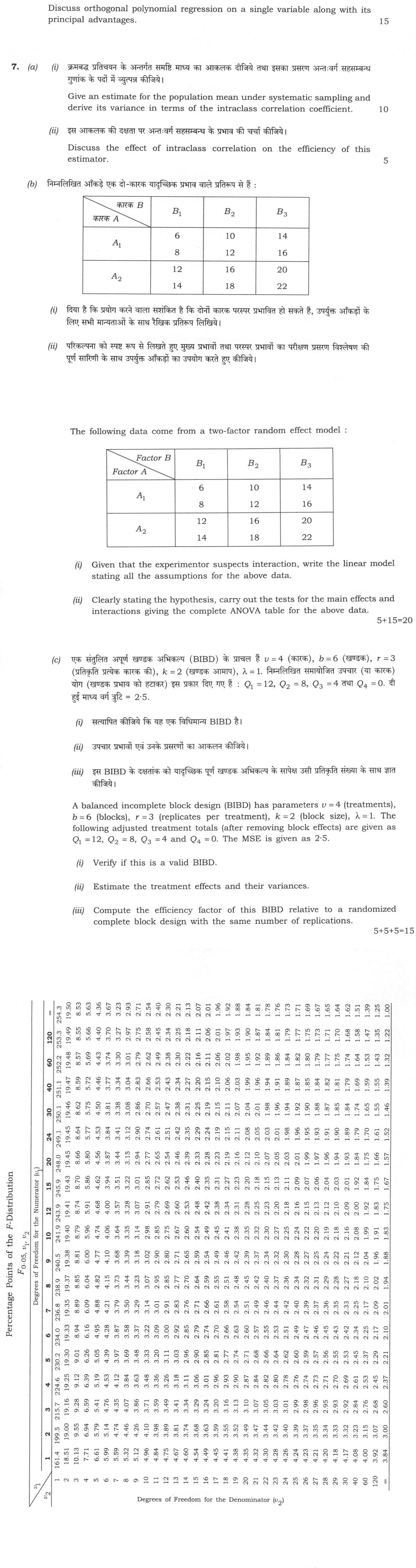
The following data are from a two-factor random effects model : | Factor B Factor A | B₁ | B₂ | B₃ | | A₁ | 6, 8 | 10, 12 | 14…
The following data are from a two-factor random effects model :
| Factor B Factor A | B₁ | B₂ | B₃ |
|---|---|---|---|
| A₁ | 6, 8 | 10, 12 | 14, 16 |
| A₂ | 12, 14 | 16, 18 | 20, 22 |
Give an estimate for the population mean under systematic sampling and derive its variance in terms of the intraclass correlation coefficient. 10 marks
Discuss the effect of intraclass correlation on the efficiency of this estimator. 5 marks
Given that the experimenter suspects that the two factors may interact with each other, write the linear model with all assumptions for the above data. 5 marks
Stating the hypothesis clearly, carry out the analysis of variance for the main effects and interaction effects using the above data, with the complete ANOVA table. 15 marks
A balanced incomplete block design (BIBD) has parameters v = 4 (treatments), b = 6 (blocks), r = 3 (replicates per treatment), k = 2 (block size), λ = 1. The following adjusted treatment totals (after removing block effects) are given as Q₁ = 12, Q₂ = 8, Q₃ = 4 and Q₄ = 0. The MSE is given as 2·5.
Verify if this is a valid BIBD.
Estimate the treatment effects and their variances.
Compute the efficiency factor of this BIBD relative to a randomized complete block design with the same number of replications. 15 marks
हिंदी में प्रश्न पढ़ें
निम्नलिखित आँकड़े एक दो-कारक यादृच्छिक प्रभाव वाले प्रतिरूप से हैं :
| कारक B कारक A | B₁ | B₂ | B₃ |
|---|---|---|---|
| A₁ | 6, 8 | 10, 12 | 14, 16 |
| A₂ | 12, 14 | 16, 18 | 20, 22 |
क्रमबद्ध प्रतिचयन के अन्तर्गत समष्टि माध्य का आकलक दीजिये तथा इसका प्रसरण अन्तःवर्ग सहसम्बन्ध गुणांक के पदों में व्युत्पन्न कीजिये। (10 अंक)
इस आकलक की दक्षता पर अन्तःवर्ग सहसम्बन्ध के प्रभाव की चर्चा कीजिये। (5 अंक)
दिया है कि प्रयोगकर्ता को संदेह है कि दोनों कारक परस्पर अन्योन्यक्रिया कर सकते हैं, उपर्युक्त आँकड़ों के लिए सभी मान्यताओं के साथ रैखिक प्रतिरूप लिखिये। (5 अंक)
परिकल्पना को स्पष्ट रूप से लिखते हुए मुख्य प्रभावों तथा परस्पर प्रभावों का परीक्षण प्रसरण विश्लेषण की पूर्ण सारणी के साथ उपर्युक्त आँकड़ों का उपयोग करते हुए कीजिये। (15 अंक)
एक संतुलित अपूर्ण खण्डक अभिकल्प (BIBD) के प्राचल हैं v = 4 (उपचार), b = 6 (खण्डक), r = 3 (प्रत्येक उपचार की प्रतिकृतियाँ), k = 2 (खण्डक आमाप), λ = 1. निम्नलिखित समायोजित उपचार (या कारक) योग (खण्डक प्रभाव को हटाकर) इस प्रकार दिए गए हैं : Q₁ = 12, Q₂ = 8, Q₃ = 4 तथा Q₄ = 0. दी हुई माध्य वर्ग त्रुटि = 2·5.
सत्यापित कीजिये कि यह एक विधिमान्य BIBD है।
उपचार प्रभावों एवं उनके प्रसरणों का आकलन कीजिये।
इस BIBD के दक्षतांक को यादृच्छिक पूर्ण खण्डक अभिकल्प के सापेक्ष उसी प्रतिकृति संख्या के साथ ज्ञात कीजिये। (15 अंक)
Model answer
Drafted with AI by UPSC Answer Check against this question's marking rubric, to the expected length. UPSC does not publish answers for Mains — this is one way to score well, not an official key. How we build rubrics and answers.
(a) (i) Systematic sampling: estimator and variance
Let N = nk units be arranged in order, n the sample size and k the sampling interval. A random start i is chosen from 1, 2, …, k and the sample is yᵢ, yᵢ₊ₖ, …, yᵢ₊₍ₙ₋₁₎ₖ. The estimator of the population mean is ȳ_sy = (1/n) Σⱼ₌₀ⁿ⁻¹ yᵢ₊ⱼₖ. Each of the k possible samples has probability 1/k, so E(ȳ_sy) = (1/k)Σᵢ ȳᵢ = Ȳ (unbiased), and V(ȳ_sy) = (1/k) Σᵢ₌₁ᵏ (ȳᵢ − Ȳ)². Write yᵢⱼ for the j-th unit of the i-th sample and σ² = Σ(y − Ȳ)²/N = (N − 1)S²/N. Then n²(ȳᵢ − Ȳ)² = Σⱼ(yᵢⱼ − Ȳ)² + Σⱼ≠l(yᵢⱼ − Ȳ)(yᵢₗ − Ȳ). Define the intraclass correlation between units of the same systematic sample ρ_w = Σᵢ Σⱼ≠l(yᵢⱼ − Ȳ)(yᵢₗ − Ȳ) / [kn(n − 1)σ²]. Averaging over the k samples, (1/k)ΣᵢΣⱼ(yᵢⱼ − Ȳ)² = Nσ²/k = nσ², so V(ȳ_sy) = (1/n²)[nσ² + n(n − 1)ρ_w σ²], i.e. V(ȳ_sy) = (σ²/n)[1 + (n − 1)ρ_w] = ((N − 1)/N)(S²/n)[1 + (n − 1)ρ_w], with −1/(n − 1) ≤ ρ_w ≤ 1.
(a) (ii) Effect of intraclass correlation on efficiency
Compare with SRSWOR, V(ȳ) = (N − n)S²/(Nn). If ρ_w > 0 (units within a sample alike) the factor [1 + (n − 1)ρ_w] exceeds 1 and systematic sampling loses precision; the worst case is a periodic population whose period equals k. If ρ_w ≈ 0 (random order) the two designs are about equally precise. If ρ_w < 0 (units within a sample dissimilar, e.g. a linear trend) systematic sampling gains. Solving (N − 1)[1 + (n − 1)ρ_w] < N − n gives the exact condition: systematic sampling is more efficient than SRSWOR iff ρ_w < −1/(N − 1); the variance becomes zero at ρ_w = −1/(n − 1). A single systematic sample gives no unbiased variance estimate, so several random starts are used in practice.
(b) (i) Two-factor random-effects model with interaction
Factor A at a = 2 levels, factor B at b = 3 levels, n = 2 observations per cell (N = 12): yᵢⱼₖ = μ + aᵢ + bⱼ + (ab)ᵢⱼ + eᵢⱼₖ, i = 1, 2; j = 1, 2, 3; k = 1, 2. Assumptions: μ is a fixed constant; aᵢ ~ N(0, σ²_A), bⱼ ~ N(0, σ²_B), (ab)ᵢⱼ ~ N(0, σ²_AB), eᵢⱼₖ ~ N(0, σ²ₑ), each set i.i.d. and all sets mutually independent (no side conditions Σaᵢ = 0 etc., as the levels are random samples of levels). Hence E(yᵢⱼₖ) = μ and V(yᵢⱼₖ) = σ²_A + σ²_B + σ²_AB + σ²ₑ.
(b) (ii) ANOVA for main effects and interaction
Hypotheses: H₀^AB: σ²_AB = 0 vs σ²_AB > 0; H₀^A: σ²_A = 0 vs σ²_A > 0; H₀^B: σ²_B = 0 vs σ²_B > 0.
G = 168, CF = 168²/12 = 2352, Σy² = 2600, so SS_T = 248. A totals 66, 102: SS_A = (66² + 102²)/6 − 2352 = 108. B totals 40, 56, 72: SS_B = (40² + 56² + 72²)/4 − 2352 = 128. Cell totals 14, 22, 30, 26, 34, 42: SS_cells = 5176/2 − 2352 = 236, so SS_AB = 236 − 108 − 128 = 0 and SS_E = 248 − 236 = 12.
| Source | d.f. | SS | MS | E(MS) (random model) | F |
|---|---|---|---|---|---|
| A | 1 | 108 | 108 | σ²ₑ + 2σ²_AB + 6σ²_A | 72.0 (vs pooled 1.5) |
| B | 2 | 128 | 64 | σ²ₑ + 2σ²_AB + 4σ²_B | 42.7 (vs pooled 1.5) |
| A × B | 2 | 0 | 0 | σ²ₑ + 2σ²_AB | 0 |
| Error | 6 | 12 | 2 | σ²ₑ | |
| Total | 11 | 248 |
Interaction: F = MS_AB/MS_E = 0/2 = 0 < F₀.₀₅(2, 6) = 5.14, not significant (the data are exactly additive). Main effects: in the random model they are tested against MS_AB, but MS_AB = 0 makes those ratios undefined. Pooling A × B with error: MS* = 12/8 = 1.5 on 8 d.f., so F_A = 108/1.5 = 72.0 > F₀.₀₅(1, 8) = 5.32 and F_B = 64/1.5 = 42.7 > F₀.₀₅(2, 8) = 4.46. Interaction absent; both main effects highly significant. Variance components: σ̂²ₑ = 2; σ̂²_AB = (0 − 2)/2 = −1, taken as 0; σ̂²_A = (108 − 0)/6 = 18; σ̂²_B = (64 − 0)/4 = 16.
(c) BIBD: validity, treatment effects and efficiency factor
(i) vr = 4 × 3 = 12 = bk = 6 × 2; λ(v − 1) = 1 × 3 = 3 = r(k − 1) = 3 × 1; b = 6 ≥ v = 4 (Fisher's inequality); k < v. The design is a valid BIBD (all C(4, 2) = 6 pairs as blocks). Note: adjusted totals must satisfy ΣQᵢ = 0, but the printed values sum to 24; we proceed with them as given (centring them, Qᵢ − 6 = 6, 2, −2, −6, would give τ̂ = 3, 1, −1, −3 with the same differences).
(ii) τ̂ᵢ = kQᵢ/(λv) = 2Qᵢ/4 = Qᵢ/2: τ̂₁ = 6, τ̂₂ = 4, τ̂₃ = 2, τ̂₄ = 0. With σ² = MSE = 2.5: V(τ̂ᵢ) = k(v − 1)σ²/(λv²) = 2 × 3 × 2.5/16 = 0.9375; V(τ̂ᵢ − τ̂ⱼ) = 2kσ²/(λv) = 2 × 2 × 2.5/4 = 2.5 (SE 1.58), the same for every pair.
(iii) Efficiency factor relative to an RBD with the same r: E = λv/(rk) = (1 × 4)/(3 × 2) = 2/3 ≈ 0.667, i.e. for equal error variance the BIBD gives 66.7% of the information of the RBD; it pays only if the smaller blocks reduce the error variance by more than one-third.
How this answer will be evaluated
Evaluation rubric
Each sub-part is marked on its own, against the marks and word limit printed on the paper.
- (a)(i) Give the usual estimator of the population mean under linear systematic sampling and derive its variance expressed in terms of the intraclass correlation coefficient ρ_w between units of the same systematic sample. 10 marks
Must cover
- N = nk, random start, k possible samples each with probability 1/k
- ȳ_sy = (1/n)Σ_j y_{i+jk}, unbiased for Ȳ when N = nk
- V(ȳ_sy) = (1/k)Σ_i(ȳ_i − Ȳ)²
- Intraclass correlation ρ_w within a systematic sample
- V(ȳ_sy) = ((N − 1)S²/(Nn))[1 + (n − 1)ρ_w]
- −1/(n − 1) ≤ ρ_w ≤ 1
Loses marks
- Quoting the SRSWOR variance (1 − f)S²/n as the systematic-sampling variance
- Using the intracluster correlation between different systematic samples instead of within the same sample
- Confusing σ² (divisor N) with S² (divisor N − 1) and so losing the (N − 1)/N factor
- Forgetting that systematic sampling has only k distinct samples, so no unbiased variance estimator exists from a single sample
- Omitting the permissible range of ρ_w, which is what guarantees V ≥ 0
Earns more
- Sets up N = nk with a random start, gives ȳ_sy = (1/n)Σ_{j=0}^{n−1} y_{i+jk} and shows E(ȳ_sy) = Ȳ (unbiased when N is a multiple of n)
- V(ȳ_sy) = (1/k)Σ_{i=1}^{k}(ȳ_i − Ȳ)², i.e. the variance is purely between the k possible systematic samples
- (a)(ii) 'Discuss the effect' — explain how the sign and magnitude of the intraclass correlation ρ_w govern the efficiency of the systematic-sampling estimator of the mean, with the precise condition under which systematic sampling beats SRSWOR. 5 marks
Must cover
- V(ȳ_sy) = (σ²/n)[1 + (n − 1)ρ_w]
- ρ_w > 0 ⇒ less efficient; ρ_w < 0 ⇒ more efficient; ρ_w ≈ 0 ⇒ comparable to SRSWOR
- Break-even condition ρ_w < −1/(N − 1)
- Periodicity matching the sampling interval k is the worst case
- Single systematic sample gives no unbiased variance estimator (use multiple random starts)
Loses marks
- Getting the direction backwards — positive intraclass correlation HURTS systematic sampling
- Saying systematic sampling is 'always' more (or always less) efficient than SRSWOR
- Quoting the break-even as ρ_w < 0 rather than the sharper ρ_w < −1/(N − 1)
- Confusing within-sample (intraclass) correlation with the between-sample variance
- Ignoring the periodicity hazard, which is the classic textbook caution
Earns more
- Gives the exact break-even condition ρ_w < −1/(N − 1) for beating SRSWOR, and notes V = 0 at the minimum ρ_w = −1/(n − 1)
- ρ_w ≈ 0 (random ordering) makes the two designs equivalent; practical advice on ordering the frame / multiple random starts for variance estimation
- (b)(i) Write the linear model, with ALL its assumptions, for the given two-factor RANDOM-effects data (Factor A at 2 levels, Factor B at 3 levels, 2 observations per cell) when the experimenter suspects an A × B interaction. Figure/table: the data are A1: (6,8), (10,12), (14,16) and A2: (12,14), (16,18), (20,22) across B1, B2, B3. 5 marks
Must cover
- y_ijk = μ + a_i + b_j + (ab)_ij + e_ijk
- i = 1,2 (a = 2); j = 1,2,3 (b = 3); k = 1,2 (n = 2); N = 12
- a_i ~ N(0, σ²_A), b_j ~ N(0, σ²_B), (ab)_ij ~ N(0, σ²_AB), e_ijk ~ N(0, σ²_e)
- Mutual independence of all random components
- V(y_ijk) = σ²_A + σ²_B + σ²_AB + σ²_e
Loses marks
- Writing the fixed-effects model with side conditions Σa_i = Σb_j = Σ(ab)_ij = 0 — those do not apply to random effects
- Omitting the interaction term when the question says the experimenter suspects interaction
- Leaving out the normality or the mutual-independence assumptions
- Using only two subscripts (y_ij) and so having no residual degrees of freedom for the replicates
- Not specifying the ranges of i, j, k for this particular 2 × 3 × 2 layout
Earns more
- Mutual independence of the four sets of random components explicitly assumed
- Consequences stated: E(y_ijk) = μ, V(y_ijk) = σ²_A + σ²_B + σ²_AB + σ²_e; hypotheses concern the variance components, and inference extends to the whole population of levels
- (b)(ii) State the hypotheses and carry out the complete two-way ANOVA with interaction for the given 2 × 3 × 2 random-effects data, presenting the full ANOVA table (sources, d.f., SS, MS, F) and the conclusions. Figure/table: A1: B1 (6,8), B2 (10,12), B3 (14,16); A2: B1 (12,14), B2 (16,18), B3 (20,22). 15 marks
Must cover
- CF = 2352; SS(Total) = 248; SS(A) = 108; SS(B) = 128; SS(AB) = 0; SS(Error) = 12
- d.f. 1, 2, 2, 6, 11; MS 108, 64, 0, 2
- Random model EMS: main effects tested against MS_AB
- F(2, 6; 0.05) = 5.14; F(1, 8; 0.05) = 5.32; F(2, 8; 0.05) = 4.46
- Interaction not significant; both main effects significant
- Variance components σ̂²_A = 18, σ̂²_B = 16, σ̂²_AB = 0, σ̂²_e = 2
Loses marks
- Using the fixed-effects F-ratios (MS_A/MS_E = 54 and MS_B/MS_E = 32) without noting that the random model requires MS_AB in the denominator
- Mis-computing SS(cells) and therefore obtaining a non-zero interaction SS
- Wrong divisors: SS(A) needs bn = 6 observations per A total and SS(B) needs an = 4 per B total
- Reporting a negative variance-component estimate (−1) without truncating it to zero or commenting on it
- Omitting the d.f. column or the total row, so the table is not the 'complete ANOVA table' asked for
Earns more
- Correction factor CF = 2352 and SS(Total) = 2600 − 2352 = 248 on 11 d.f.
- Complete ANOVA table with MS values 108, 64, 0 and MSE = 2, and the interaction test F_AB = 0 against F(2,6;0.05) = 5.14 — not significant
- Main-effect tests handled correctly for a random model (EMS ⇒ test against MS_AB; MS_AB = 0 so pool to MS = 1.5 on 8 d.f., giving F_A = 72.0 and F_B = 42.7, both significant) plus variance components σ̂²_A = 18, σ̂²_B = 16, σ̂²_AB = 0, σ̂²_e = 2
- (c) Three demands for the BIBD with v = 4, b = 6, r = 3, k = 2, λ = 1, adjusted treatment totals Q1 = 12, Q2 = 8, Q3 = 4, Q4 = 0 and MSE = 2.5: (i) verify the parameter relations, (ii) estimate the treatment effects and their variances, and (iii) compute the efficiency factor relative to an RBD with the same number of replications. 15 marks
Must cover
- vr = bk = 12; λ(v − 1) = r(k − 1) = 3; b ≥ v (Fisher's inequality)
- τ̂_i = kQ_i/(λv) = Q_i/2
- τ̂ = (6, 4, 2, 0)
- V(τ̂_i) = k(v − 1)σ²/(λv²) = 0.9375; V(τ̂_i − τ̂_j) = 2kσ²/(λv) = 2.5
- Efficiency factor E = λv/(rk) = 2/3 = 0.667
- ΣQ_i = 0 is a required property of adjusted treatment totals
Loses marks
- Using τ̂_i = Q_i/r or Q_i/λ instead of kQ_i/(λv)
- Computing the efficiency factor as rk/(λv) = 1.5 (the reciprocal) and claiming the BIBD is more efficient
- Quoting V(τ̂_i − τ̂_j) = 2σ²/r (the RBD formula) instead of 2kσ²/(λv)
- Checking only vr = bk and declaring the design valid without the λ(v−1) = r(k−1) relation or Fisher's inequality
- Forgetting that MSE = 2.5 plays the role of σ² in all the variance formulae
Earns more
- Variances V(τ̂_i) = k(v − 1)σ²/(λv²) = 2(3)(2.5)/16 = 0.9375 and V(τ̂_i − τ̂_j) = 2kσ²/(λv) = 2.5 (SE of a difference 1.58), constant over all pairs
- Notes the internal inconsistency that ΣQ_i should be 0 for a BIBD but the given Q values sum to 24
What "Calculate" is asking you to do
Apply the standard formula or schedule to data the question has already supplied — a table of readings, cost records, a balance sheet — and produce the number. The method is rarely in doubt; the marks sit in the named intermediate quantities, each of which has to appear as a labelled line.
Structure that answers it
Data as given → formula or standard treatment, named → substitution → each intermediate, labelled → result with units
Where marks are lost
Omitting an intermediate the marking scheme pays for separately, or rounding at an intermediate line so the final figure drifts. In commerce and accountancy, any figure in a statement that no numbered working note supports is treated as unearned.
Practice this exact question
Write your answer and it is marked point by point against the model answer above — what you covered, what you missed, what you got wrong.
Evaluate my answer →More from Statistics 2026 Paper I
- Q4 (a) Let X₁, X₂, ⋯, Xₙ be i.i.d. random variables following N(μ, σ²). Find the maximum lik…
- Q5 (a) Let Y₁, Y₂, ⋯, Yₙ be n independent observations from a population with mean μ and var…
- Q6 (a) Let l′β be any estimable linear function of parameters β₁, β₂, ⋯, β_p. Then prove tha…
- Q7 The following data are from a two-factor random effects model : | Factor B \ Factor A | B…
- Q8 (a) Define multivariate normal distribution and write down its important properties. Let…