Paper I — Q6
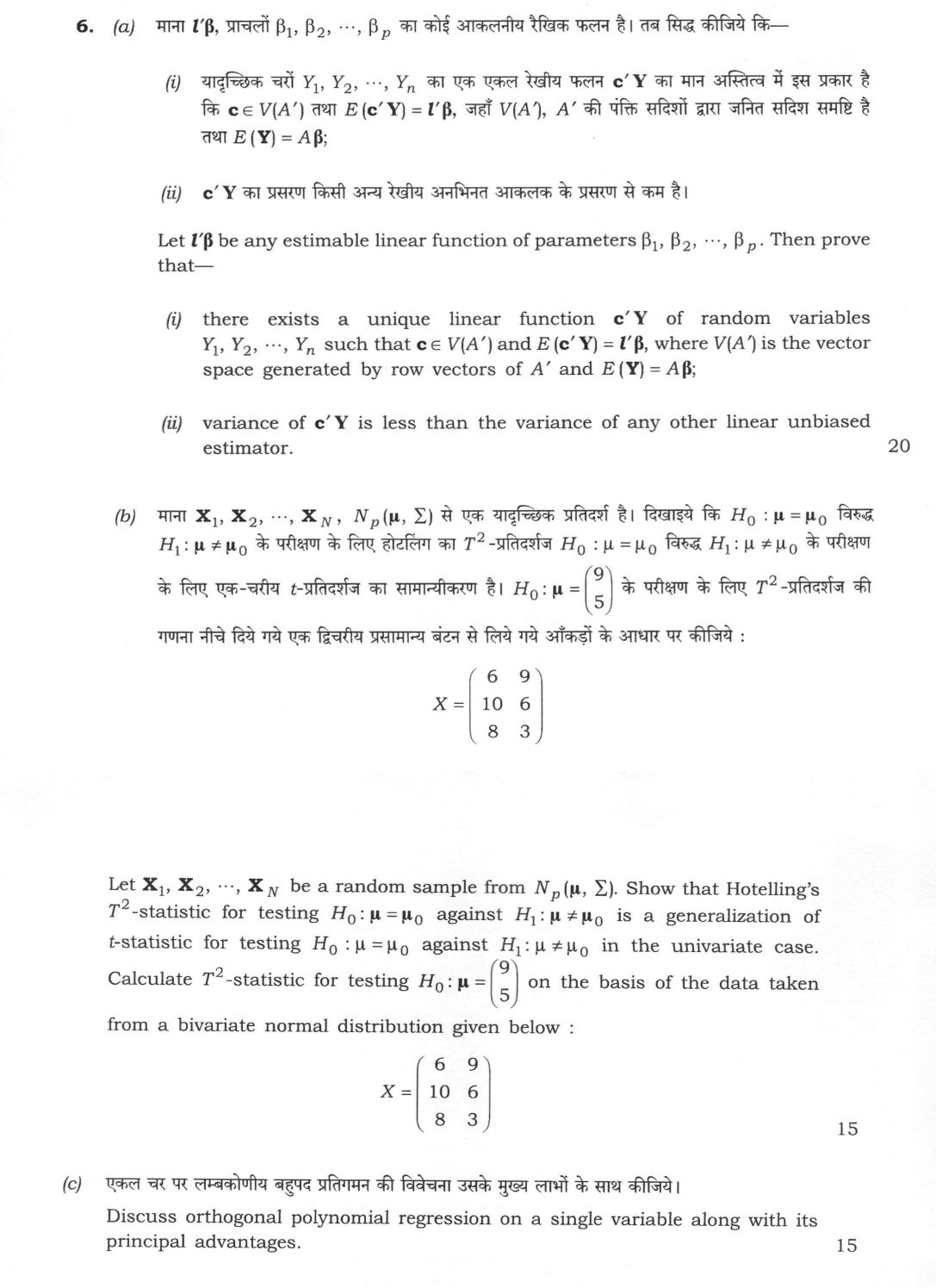
(a) Let l′β be any estimable linear function of parameters β₁, β₂, ⋯, β_p. Then prove that— (i) there exists a unique linear…
Let l′β be any estimable linear function of parameters β₁, β₂, ⋯, β_p. Then prove that—
there exists a unique linear function c′Y of random variables Y₁, Y₂, ⋯, Y_n such that c ∈ V(A′) and E(c′Y) = l′β, where V(A′) is the vector space generated by row vectors of A′ and E(Y) = Aβ;
variance of c′Y is less than the variance of any other linear unbiased estimator. 20 marks
Let X₁, X₂, ⋯, X_N be a random sample from N_p(μ, Σ). Show that Hotelling's T²-statistic for testing H₀ : μ = μ₀ against H₁ : μ ≠ μ₀ is a generalization of t-statistic for testing H₀ : μ = μ₀ against H₁ : μ ≠ μ₀ in the univariate case. Calculate T²-statistic for testing H₀ : μ = ( 9 , 5 ) on the basis of the data taken from a bivariate normal distribution given below : X = [ 6 9 ; 10 6 ; 8 3 ] 15 marks
Discuss orthogonal polynomial regression on a single variable along with its principal advantages. 15 marks
हिंदी में प्रश्न पढ़ें
माना l′β, प्राचलों β₁, β₂, ⋯, β_p का कोई आकलनीय रैखिक फलन है। तब सिद्ध कीजिये कि—
यादृच्छिक चरों Y₁, Y₂, ⋯, Y_n का एक एकल रेखीय फलन c′Y का मान अस्तित्व में इस प्रकार है कि c ∈ V(A′) तथा E(c′Y) = l′β, जहाँ V(A′), A′ की पंक्ति सदिशों द्वारा जनित सदिश समष्टि है तथा E(Y) = Aβ;
c′Y का प्रसरण किसी अन्य रेखीय अनभिनत आकलक के प्रसरण से कम है। (20 अंक)
मान लीजिए X₁, X₂, ⋯, X_N, N_p(μ, Σ) से एक यादृच्छिक प्रतिदर्श है। दर्शाइये कि H₀ : μ = μ₀ के विरुद्ध H₁ : μ ≠ μ₀ के परीक्षण के लिए हॉटलिंग की T²-सांख्यिकी, एक चर वाले प्रकरण में H₀ : μ = μ₀ के विरुद्ध H₁ : μ ≠ μ₀ के परीक्षण के लिए t-सांख्यिकी का सामान्यीकरण है। नीचे दिये गये द्विचर सामान्य बंटन से लिये गये आँकड़ों के आधार पर H₀ : μ = ( 9 , 5 ) के परीक्षण के लिए T²-सांख्यिकी की गणना कीजिये : X = [ 6 9 ; 10 6 ; 8 3 ] (15 अंक)
एकल चर पर लम्बकोणीय बहुपद प्रतिगमन की विवेचना उसके मुख्य लाभों के साथ कीजिये। (15 अंक)
Model answer
Drafted with AI by UPSC Answer Check against this question's marking rubric, to the expected length. UPSC does not publish answers for Mains — this is one way to score well, not an official key. How we build rubrics and answers.
(a) Existence, uniqueness and minimum variance of c′Y
Set-up: E(Y) = Aβ, A of order n × p, D(Y) = σ²Iₙ. V(A′) is the space spanned by the rows of A′, i.e. the column space of A; its orthogonal complement is {v : A′v = 0}.
(i) Existence. l′β is estimable, so some linear function d′Y has E(d′Y) = d′Aβ = l′β for all β, i.e. A′d = l. Write d = c + e, where c is the orthogonal projection of d on V(A′) and e ⊥ V(A′), so A′e = 0. Then A′c = A′d = l and E(c′Y) = c′Aβ = (A′c)′β = l′β, with c ∈ V(A′). Uniqueness. Suppose c₁, c₂ ∈ V(A′) both give E(cᵢ′Y) = l′β. Then A′(c₁ − c₂) = 0, so c₁ − c₂ ⊥ V(A′); but c₁ − c₂ ∈ V(A′). A vector orthogonal to itself is zero, so c₁ = c₂: c′Y is unique.
(ii) Let d′Y be any linear unbiased estimator of l′β, so A′d = l and A′(d − c) = 0. Since c ∈ V(A′), c = Aw for some w, and c′(d − c) = w′A′(d − c) = 0. Hence V(d′Y) = σ² d′d = σ²[c + (d − c)]′[c + (d − c)] = σ² c′c + σ²(d − c)′(d − c) ≥ σ² c′c = V(c′Y), with equality only when d = c. c′Y has smaller variance than any other linear unbiased estimator: it is the BLUE of l′β (Gauss-Markov theorem). It also equals l′β̂ for any solution β̂ of the normal equations A′Aβ̂ = A′Y.
(b) Hotelling's T² as a generalisation of t, and its computation
For X₁, …, X_N from N_p(μ, Σ), with X̄ the mean vector and S = Σ(Xᵢ − X̄)(Xᵢ − X̄)′/(N − 1), T² = N(X̄ − μ₀)′ S⁻¹ (X̄ − μ₀), and (N − p)T²/[p(N − 1)] ~ F(p, N − p) under H₀. For p = 1, X̄ = x̄ and S = s², so T² = N(x̄ − μ₀)²/s² = [√N(x̄ − μ₀)/s]² = t², the square of Student's t with N − 1 d.f. (the two-sided t-test). Also T² = max over a of the squared t-statistic for a′X, so it is the natural multivariate extension.
Computation (N = 3, p = 2), observations (6, 9), (10, 6), (8, 3): X̄ = ((6 + 10 + 8)/3, (9 + 6 + 3)/3)′ = (8, 6)′. Deviations: (−2, 3), (2, 0), (0, −3). SS₁₁ = 4 + 4 + 0 = 8; SS₂₂ = 9 + 0 + 9 = 18; SP₁₂ = −6 + 0 + 0 = −6. S = (1/2)[8 −6; −6 18] = [4 −3; −3 9]; |S| = 36 − 9 = 27; S⁻¹ = (1/27)[9 3; 3 4]. X̄ − μ₀ = (8 − 9, 6 − 5)′ = (−1, 1)′. (X̄ − μ₀)′S⁻¹(X̄ − μ₀) = (1/27)[9(1) + 2·3(−1)(1) + 4(1)] = 7/27. T² = 3 × 7/27 = 7/9 ≈ 0.778. F = (N − p)T²/[p(N − 1)] = (1 × 7/9)/(2 × 2) = 7/36 ≈ 0.19, far below F₀.₀₅(2, 1) = 199.5, so H₀: μ = (9, 5)′ is not rejected.
(c) Orthogonal polynomial regression on a single variable
To fit a polynomial of degree k in x, instead of the powers 1, x, x², … we use polynomials ξ₀(x) = 1, ξ₁(x), …, ξ_k(x), ξⱼ of degree j, chosen to be orthogonal over the observed points: Σᵢ ξⱼ(xᵢ)ξ_r(xᵢ) = 0 for j ≠ r. The model is y = β₀ξ₀(x) + β₁ξ₁(x) + … + β_kξ_k(x) + e.
Construction: apply Gram-Schmidt to 1, x, x², … over the design points. For equally spaced x the values are tabulated (Fisher-Yates tables); e.g. for x = 1, …, 5, ξ₁ = x − 3 gives −2, −1, 0, 1, 2 and ξ₂ = (x − 3)² − 2 gives 2, −1, −2, −1, 2.
Estimation: because X′X is diagonal, β̂ⱼ = Σ yᵢξⱼ(xᵢ)/Σ ξⱼ²(xᵢ), with V(β̂ⱼ) = σ²/Σ ξⱼ²(xᵢ) and Cov(β̂ⱼ, β̂_r) = 0.
Principal advantages:
- Adding a higher-degree term leaves all earlier estimates unchanged, so the degree can be raised step by step.
- The regression SS splits into independent components β̂ⱼ² Σ ξⱼ²(xᵢ), one per degree, so the linear, quadratic, cubic … effects are tested separately by F-tests in one ANOVA table.
- The estimates are uncorrelated and easy to compute by hand.
- The normal equations are perfectly conditioned; raw powers x, x², x³ are highly collinear and give unstable, rounding-sensitive coefficients.
Limitations: the coefficients refer to ξⱼ, so converting to powers of x needs extra algebra, and the tables apply only to equally spaced x (otherwise the polynomials must be constructed for the data). The method is therefore the standard tool for trend analysis of quantitative factor levels in designed experiments.
How this answer will be evaluated
What earns full marks: Rigorous proofs, correct computations, clear interpretation of all parts
Evaluation rubric
Each sub-part is marked on its own, against the marks and word limit printed on the paper.
- (a) Prove, for the linear model E(Y) = Aβ with D(Y) = σ²I and an estimable l′β: (i) existence and uniqueness of a linear function c′Y with c ∈ V(A′) (the column space of A) and E(c′Y) = l′β; (ii) that its variance is smaller than that of any other linear unbiased estimator of l′β (Gauss-Markov). 20 marks
derive— given → assumptions → stepwise derivation → result → check
Must cover
- Estimability: some d′Y has E(d′Y) = l′β, i.e. A′d = l
- Existence: c = projection of d on V(A′) satisfies A′c = l, so E(c′Y) = l′β
- Uniqueness: c₁, c₂ ∈ V(A′) with A′c₁ = A′c₂ = l ⇒ c₁ − c₂ lies in V(A′) and is orthogonal to it ⇒ c₁ = c₂
- For any unbiased d′Y: A′(d − c) = 0 ⇒ c′(d − c) = 0 ⇒ V(d′Y) = σ²c′c + σ²(d − c)′(d − c) ≥ V(c′Y)
- Equality iff d = c, so c′Y is the unique BLUE
Loses marks
- Asserting uniqueness or minimum variance without proof ('by the Gauss-Markov theorem')
- Confusing V(A′) with the parameter space or with the column space of A′
- Omitting D(Y) = σ²I, or dropping the cross term c′(d − c) without showing it is zero
Earns more
- States D(Y) = σ²I explicitly (needed for (ii))
- Identifies V(A′) as the column space of A and its orthogonal complement as {v : A′v = 0}
Extra mark
- Remarks that c′Y = l′β̂ for any solution β̂ of the normal equations A′Aβ̂ = A′Y
- (b) Show that Hotelling's T² = N(X̄ − μ₀)′S⁻¹(X̄ − μ₀) reduces to the square of Student's t when p = 1, and calculate T² for H₀: μ = (9, 5)′ from the three bivariate observations (6, 9), (10, 6), (8, 3). 15 marks
calculate— given → formula → substitution → result with units → interpretation
Must cover
- T² = N(X̄ − μ₀)′S⁻¹(X̄ − μ₀) with S = Σ(Xᵢ − X̄)(Xᵢ − X̄)′/(N − 1)
- p = 1: T² = N(x̄ − μ₀)²/s² = t² with N − 1 d.f.
- X̄ = (8, 6)′, S = [4 −3; −3 9], |S| = 27
- S⁻¹ = (1/27)[9 3; 3 4], X̄ − μ₀ = (−1, 1)′
- T² = 3 × 7/27 = 7/9 ≈ 0.778
Loses marks
- Using divisor N instead of N − 1 in S (gives T² = 7/6) without saying so
- Inverting S with wrong off-diagonal signs (e.g. [9 −3; −3 4]/27, giving 19/9) or taking |S| = 45
- Omitting the univariate reduction, or stating it without showing T² = t²
Earns more
- Notes that T² is the maximum over a of the squared univariate t for a′X (union-intersection view)
- Converts to F = (N − p)T²/[p(N − 1)] = 7/36 ≈ 0.19 on (2, 1) d.f., far below F₀.₀₅(2, 1) = 199.5, so H₀ is not rejected
Extra mark
- Mentions that T² is also the likelihood-ratio test and is invariant under nonsingular linear transformations
- (c) Discuss fitting a polynomial regression in one variable by orthogonal polynomials — construction, estimation, testing of successive degrees — and its principal advantages over the ordinary power-series fit. 15 marks
discuss— intro → 3-4 dimensions → example → balanced close
Must cover
- Model y = Σ βⱼξⱼ(x) + e with Σᵢ ξⱼ(xᵢ)ξ_r(xᵢ) = 0 for j ≠ r
- Construction by Gram-Schmidt on 1, x, x², … over the design points; tabulated values for equally spaced x
- β̂ⱼ = Σyᵢξⱼ(xᵢ)/Σξⱼ²(xᵢ), V(β̂ⱼ) = σ²/Σξⱼ²(xᵢ), estimates uncorrelated
- Advantages: earlier estimates unchanged when a degree is added; SS for each degree separates in ANOVA; no multicollinearity
Loses marks
- Confusing orthogonal polynomials with orthogonal arrays or orthogonal designs
- Listing advantages without explaining that they follow from X′X being diagonal
Earns more
- Worked illustration, e.g. x = 1, …, 5: ξ₁ = x − 3, ξ₂ = (x − 3)² − 2
- Contrast with the raw-power fit (ill-conditioned X′X; all coefficients change when a term is added)
Extra mark
- Notes limitations: coefficients must be converted back to powers of x; tables only for equally spaced x
What "Prove" is asking you to do
Establish that the statement holds for every case it claims, not for one representative case. The argument must be closed: each line follows from a definition, a hypothesis, or a named theorem you are entitled to use.
Structure that answers it
Given and to prove, restated → theorem or construction to be used, named → the argument line by line → conclusion stated as proved
Where marks are lost
Testing one example, which illustrates but proves nothing. On an if and only if claim, proving one direction and stopping forfeits that half outright, and degenerate cases — zero, the empty set, the equality case — have to be disposed of rather than assumed away.
Practice this exact question
Write your answer and it is marked point by point against the model answer above — what you covered, what you missed, what you got wrong.
Evaluate my answer →More from Statistics 2026 Paper I
- Q3 (a) Let the joint probability density function of X and Y be f(x, y) = 3/4 ( xy + x²/2 )…
- Q4 (a) Let X₁, X₂, ⋯, Xₙ be i.i.d. random variables following N(μ, σ²). Find the maximum lik…
- Q5 (a) Let Y₁, Y₂, ⋯, Yₙ be n independent observations from a population with mean μ and var…
- Q6 (a) Let l′β be any estimable linear function of parameters β₁, β₂, ⋯, β_p. Then prove tha…
- Q7 The following data are from a two-factor random effects model : | Factor B \ Factor A | B…
- Q8 (a) Define multivariate normal distribution and write down its important properties. Let…