Paper I — Q5
(a) Let Y₁, Y₂, ⋯, Yₙ be n independent observations from a population with mean μ and variance σ². Obtain the best linear…
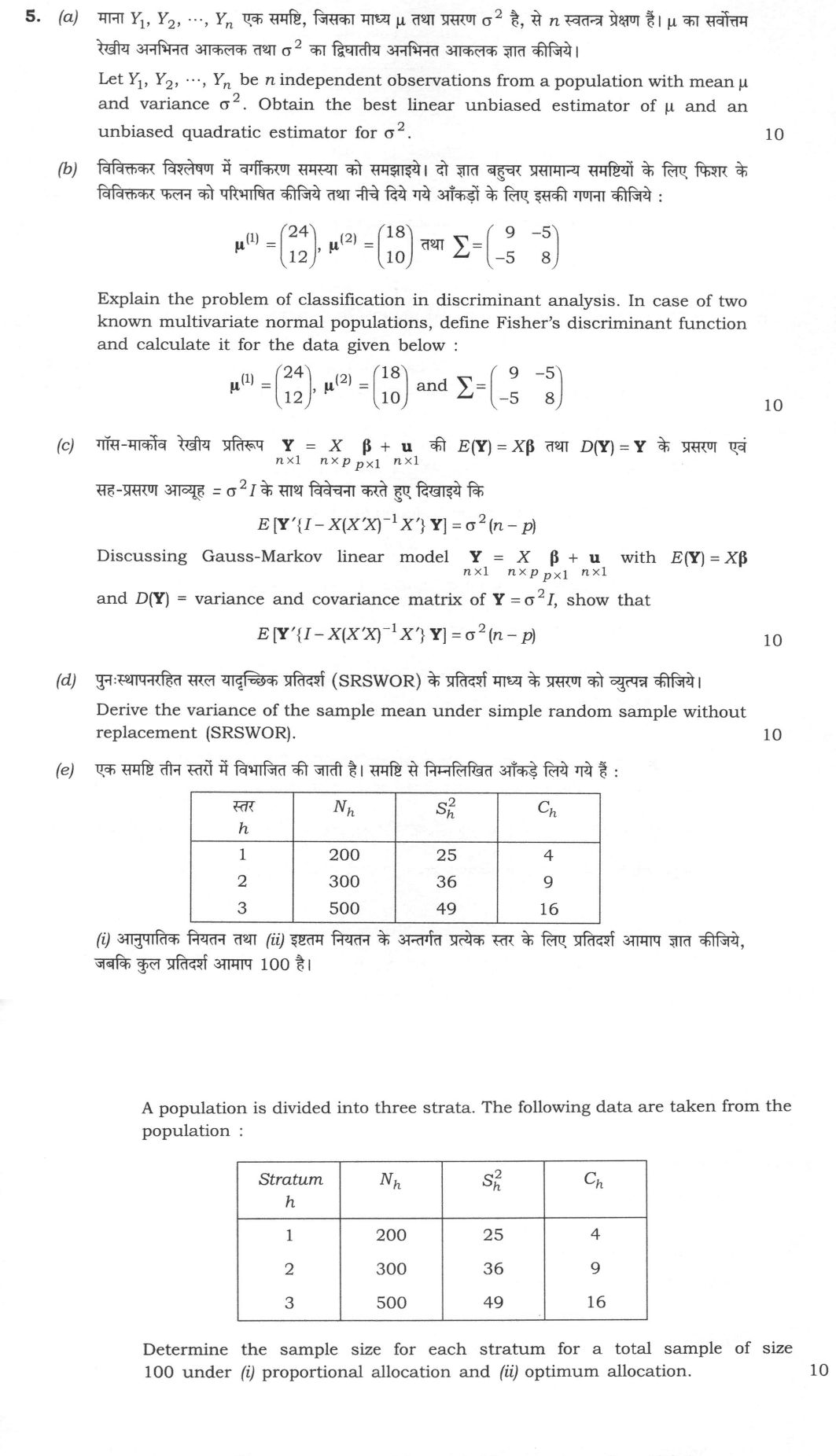
Let Y₁, Y₂, ⋯, Yₙ be n independent observations from a population with mean μ and variance σ². Obtain the best linear unbiased estimator of μ and an unbiased quadratic estimator for σ². 10 marks
Explain the problem of classification in discriminant analysis. In case of two known multivariate normal populations, define Fisher's discriminant function and calculate it for the data given below : μ⁽¹⁾ = (24, 12), μ⁽²⁾ = (18, 10) and Σ = (9 −5; −5 8) 10 marks
Discussing Gauss–Markov linear model Yₙ×1 = Xₙ×p βₚ×1 + uₙ×1 with E(Y) = Xβ and D(Y) = variance and covariance matrix of Y = σ²I, show that E[Y′I − X(X′X)⁻¹X′Y] = σ²(n − p) 10 marks
Derive the variance of the sample mean under simple random sample without replacement (SRSWOR). 10 marks
A population is divided into three strata. The following data are taken from the population :
| Stratum h | Nₕ | Sₕ² | Cₕ |
|---|---|---|---|
| 1 | 200 | 25 | 4 |
| 2 | 300 | 36 | 9 |
| 3 | 500 | 49 | 16 |
Determine the sample size for each stratum for a total sample of size 100 under (i) proportional allocation and (ii) optimum allocation. 10 marks
हिंदी में प्रश्न पढ़ें
माना Y₁, Y₂, ⋯, Yₙ एक समष्टि, जिसका माध्य μ तथा प्रसरण σ² है, से n स्वतन्त्र प्रेक्षण हैं। μ का सर्वोत्तम रैखीय अनभिनत आकलक तथा σ² का द्विघातीय अनभिनत आकलक ज्ञात कीजिये। (10 अंक)
विविक्तकर विश्लेषण में वर्गीकरण समस्या को समझाइये। दो ज्ञात बहुचर प्रसामान्य समष्टियों के लिए फिशर के विविक्तकर फलन को परिभाषित कीजिये तथा नीचे दिये गये आँकड़ों के लिए इसकी गणना कीजिये : μ⁽¹⁾ = (24, 12), μ⁽²⁾ = (18, 10) तथा Σ = (9 −5; −5 8) (10 अंक)
गॉस–मार्कोव रैखीय प्रतिरूप Yₙ×1 = Xₙ×p βₚ×1 + uₙ×1 की E(Y) = Xβ तथा D(Y) = Y के प्रसरण एवं सह-प्रसरण आव्यूह = σ²I के साथ विवेचना करते हुए दिखाइये कि E[Y′I − X(X′X)⁻¹X′Y] = σ²(n − p) (10 अंक)
पुन:स्थापनरहित सरल यादृच्छिक प्रतिदर्श (SRSWOR) के प्रतिदर्श माध्य के प्रसरण को व्युत्पन्न कीजिये। (10 अंक)
एक समष्टि तीन स्तरों में विभाजित की जाती है। समष्टि से निम्नलिखित आँकड़े लिये गये हैं :
| स्तर h | Nₕ | Sₕ² | Cₕ |
|---|---|---|---|
| 1 | 200 | 25 | 4 |
| 2 | 300 | 36 | 9 |
| 3 | 500 | 49 | 16 |
आनुपातिक नियतन तथा (ii) इष्टतम नियतन के अन्तर्गत प्रत्येक स्तर के लिए प्रतिदर्श आमाप ज्ञात कीजिये, जबकि कुल प्रतिदर्श आमाप 100 है। (10 अंक)
Model answer
Drafted with AI by UPSC Answer Check against this question's marking rubric, to the expected length. UPSC does not publish answers for Mains — this is one way to score well, not an official key. How we build rubrics and answers.
(a) BLUE of μ and unbiased quadratic estimator of σ²
Let T = Σaᵢ Yᵢ be any linear estimator. E(T) = μ Σaᵢ, so T is unbiased iff Σaᵢ = 1. By independence, V(T) = σ² Σaᵢ². By the Cauchy-Schwarz inequality, 1 = (Σaᵢ)² ≤ n Σaᵢ², so Σaᵢ² ≥ 1/n, with equality iff a₁ = … = aₙ = 1/n. Hence the BLUE of μ is Ȳ = (1/n)ΣYᵢ, with V(Ȳ) = σ²/n.
For σ², take the quadratic form Σ(Yᵢ − Ȳ)² = ΣYᵢ² − nȲ². Since E(Yᵢ²) = σ² + μ² and E(Ȳ²) = σ²/n + μ², E[Σ(Yᵢ − Ȳ)²] = n(σ² + μ²) − (σ² + nμ²) = (n − 1)σ². So s² = Σ(Yᵢ − Ȳ)²/(n − 1) is an unbiased quadratic estimator of σ². Only the first two moments and independence are used; normality is not needed.
(b) Classification problem and Fisher's discriminant function
The classification problem: an individual with measurement vector x is known to come from one of two (or more) populations π₁, π₂; we must divide the sample space into regions R₁, R₂ and assign x to πᵢ if x ∈ Rᵢ, so that the probabilities (or expected costs) of misclassification P(2 | 1) and P(1 | 2) are as small as possible.
Fisher's linear discriminant function: for two populations Nₚ(μ⁽¹⁾, Σ) and Nₚ(μ⁽²⁾, Σ) with common Σ, choose the linear combination a′x that maximises (a′δ)²/(a′Σa), δ = μ⁽¹⁾ − μ⁽²⁾. The solution is a ∝ Σ⁻¹δ, giving U(x) = (μ⁽¹⁾ − μ⁽²⁾)′ Σ⁻¹ x; assign x to π₁ if U(x) ≥ ½(μ⁽¹⁾ + μ⁽²⁾)′ Σ⁻¹(μ⁽¹⁾ − μ⁽²⁾), otherwise to π₂.
Computation: δ = (24 − 18, 12 − 10)′ = (6, 2)′. |Σ| = 9·8 − (−5)² = 72 − 25 = 47, and Σ⁻¹ = (1/47) [8 5; 5 9]. Σ⁻¹δ = (1/47)(8·6 + 5·2, 5·6 + 9·2)′ = (1/47)(58, 48)′. U(x) = (58x₁ + 48x₂)/47 ≈ 1.234x₁ + 1.021x₂. Cut-off: the midpoint of the means is (21, 11)′, so U = (58·21 + 48·11)/47 = 1746/47 ≈ 37.15. Assign x to π₁ if U(x) ≥ 37.15, otherwise to π₂. Mahalanobis distance D² = δ′Σ⁻¹δ = (6·58 + 2·48)/47 = 444/47 ≈ 9.45, so each misclassification probability is Φ(−D/2) ≈ 0.062.
(c) Expectation of the residual sum of squares
Model: Y = Xβ + u, E(u) = 0, D(Y) = σ²I, rank(X) = p. Let H = X(X′X)⁻¹X′ and M = I − H. H′ = H and H² = X(X′X)⁻¹X′X(X′X)⁻¹X′ = H, so H, and hence M, are symmetric idempotent. For any symmetric A, E(Y′AY) = tr(A D(Y)) + (EY)′A(EY). With A = M: Second term: β′X′MXβ = 0, because MX = X − X(X′X)⁻¹X′X = 0. First term: tr(Mσ²I) = σ² tr(M) = σ²[n − tr(X(X′X)⁻¹X′)] = σ²[n − tr((X′X)⁻¹X′X)] = σ²[n − tr(Iₚ)] = σ²(n − p). Hence E[Y′I − X(X′X)⁻¹X′Y] = σ²(n − p), so the residual mean square Y′MY/(n − p) is an unbiased estimator of σ².
(d) Variance of the sample mean under SRSWOR
Population values Y₁, …, Y_N with mean Ȳ, σ² = Σ(Yᵢ − Ȳ)²/N and S² = Σ(Yᵢ − Ȳ)²/(N − 1), so σ² = (N − 1)S²/N. Let y₁, …, yₙ be the sample drawn without replacement. Each draw yᵢ takes every population value with probability 1/N, so E(yᵢ) = Ȳ (hence E(ȳ) = Ȳ) and V(yᵢ) = σ². For i ≠ j, the pair (yᵢ, yⱼ) takes each ordered pair of distinct units with probability 1/[N(N − 1)], so Cov(yᵢ, yⱼ) = Σₖ≠l(Yₖ − Ȳ)(Yₗ − Ȳ)/[N(N − 1)] = −Σ(Yₖ − Ȳ)²/[N(N − 1)] = −σ²/(N − 1) = −S²/N, using Σₖ≠l(Yₖ − Ȳ)(Yₗ − Ȳ) = [Σ(Yₖ − Ȳ)]² − Σ(Yₖ − Ȳ)² = −Σ(Yₖ − Ȳ)². Therefore V(ȳ) = (1/n²)[Σ V(yᵢ) + Σᵢ≠j Cov(yᵢ, yⱼ)] = (1/n²)[n(N − 1)S²/N − n(n − 1)S²/N] = (N − n)S²/(Nn). V(ȳ) = ((N − n)/(Nn)) S² = (1 − f) S²/n, where f = n/N and (1 − f) is the finite population correction. An unbiased estimator is v(ȳ) = (1 − f)s²/n.
(e) Proportional and optimum allocation
N = 200 + 300 + 500 = 1000, n = 100; Sₕ = 5, 6, 7; √Cₕ = 2, 3, 4.
(i) Proportional allocation, nₕ = n Nₕ/N: n₁ = 20, n₂ = 30, n₃ = 50.
(ii) Optimum allocation with costs (minimising V(ȳ_st) for a fixed cost C = c₀ + ΣCₕ nₕ): nₕ ∝ Nₕ Sₕ/√Cₕ.
| Stratum | Nₕ | Sₕ | √Cₕ | Nₕ Sₕ/√Cₕ | nₕ = 100 × share |
|---|---|---|---|---|---|
| 1 | 200 | 5 | 2 | 500 | 25.32 |
| 2 | 300 | 6 | 3 | 600 | 30.38 |
| 3 | 500 | 7 | 4 | 875 | 44.30 |
| Total | 1000 | 1975 | 100 |
Rounding so that the total is 100 (largest remainder): n₁ = 25, n₂ = 31, n₃ = 44 (25, 30, 45 is also acceptable). The costlier third stratum gets fewer units than under proportional allocation.
How this answer will be evaluated
Evaluation rubric
Each sub-part is marked on its own, against the marks and word limit printed on the paper.
- (a) Two demands for n independent observations with common mean μ and common variance σ²: obtain the best linear unbiased estimator (BLUE) of μ, and obtain an unbiased quadratic estimator of σ². Both derivations are needed — quoting Ȳ and s² without proof is not enough. 10 marks
Must cover
- Σa_i = 1 (unbiasedness) and V(Σa_iY_i) = σ²Σa_i²
- a_i = 1/n; BLUE = Ȳ
- V(Ȳ) = σ²/n
- E[Σ(Yi − Ȳ)²] = (n − 1)σ²
- s² = Σ(Yi − Ȳ)²/(n − 1) unbiased for σ²
- Gauss-Markov setting: no normality required
Loses marks
- Asserting Ȳ is the BLUE by quoting the Gauss-Markov theorem without carrying out the constrained minimisation the question asks for
- Dividing by n instead of n − 1 in the quadratic estimator, which makes it biased
- Forgetting the independence assumption, which is what kills the cross terms in V(Σa_iY_i)
- Assuming normality — the result needs only the first two moments
- Failing to show why Σa_i² is minimised at a_i = 1/n (a mere assertion loses the 3 marks)
Earns more
- Sets up the linear class T = Σa_iY_i and derives the unbiasedness constraint Σa_i = 1, with V(T) = σ²Σa_i²
- (b) Three demands: explain what the classification problem in discriminant analysis is; define Fisher's linear discriminant function for two known multivariate normal populations with a common dispersion matrix; and compute it numerically for μ⁽¹⁾ = (24, 12)', μ⁽²⁾ = (18, 10)' and Σ = [[9, −5], [−5, 8]]. 10 marks
Must cover
- Misclassification probabilities P(2|1), P(1|2); regions R1, R2
- U = (μ⁽¹⁾ − μ⁽²⁾)'Σ⁻¹X
- |Σ| = 47, Σ⁻¹ = (1/47)[[8, 5], [5, 9]]
- U(x) = (58x1 + 48x2)/47 ≈ 1.234x1 + 1.021x2
- Cut-off = (1/2)(μ⁽¹⁾+μ⁽²⁾)'Σ⁻¹(μ⁽¹⁾−μ⁽²⁾) = 1746/47 = 37.1
- Mahalanobis distance D² = 444/47 = 9.45
Loses marks
- Inverting Σ wrongly — the off-diagonal entries of the adjugate keep the sign +5, not −5, since Σ⁻¹ = (1/|Σ|)[[σ22, −σ12], [−σ12, σ11]] with σ12 = −5
- Computing |Σ| as 72 + 25 = 97 instead of 72 − 25 = 47
- Giving only the coefficient vector and never writing the discriminant function or the classification rule
- Omitting the cut-off constant, so the rule cannot actually be applied
- Confusing Fisher's LDF with the quadratic discriminant (which arises only when the two dispersion matrices differ)
Earns more
- Correct inverse: |Σ| = 47 and Σ⁻¹ = (1/47)[[8, 5], [5, 9]]; μ⁽¹⁾ − μ⁽²⁾ = (6, 2)'
- (c) Within the Gauss-Markov set-up Y = Xβ + u with E(Y) = Xβ and D(Y) = σ²I, prove that E[Y'{I − X(X'X)⁻¹X'}Y] = σ²(n − p) — the result that makes the residual mean square an unbiased estimator of σ². 10 marks
Must cover
- Hat matrix H = X(X'X)⁻¹X', symmetric and idempotent
- E(Y'AY) = tr(A D(Y)) + (EY)'A(EY)
- (I − H)X = 0
- tr(AB) = tr(BA); tr(H) = p; tr(I − H) = n − p
- σ̂² = RSS/(n − p) is unbiased for σ²
Loses marks
- Getting tr(H) = n instead of p by not using the cyclic property of the trace
- Forgetting the mean-vector term β'X'(I−H)Xβ altogether instead of showing that it is zero
- Assuming normality of u — the result needs only the first two moments
- Writing D(Y) = σ² (a scalar) and dropping the identity matrix, which breaks the trace computation
- Not stating the full-column-rank condition needed for (X'X)⁻¹ to exist
Earns more
- States the Gauss-Markov model and assumptions (E(u) = 0, D(u) = σ²I, rank(X) = p) and identifies Y'(I − H)Y as the residual sum of squares
- Shows H = X(X'X)⁻¹X' is symmetric and idempotent, hence so is M = I − H
- (d) Derive — not merely quote — the variance of the sample mean ȳ under simple random sampling without replacement, ending with V(ȳ) = ((N − n)/(Nn))S² = (1 − f)S²/n. 10 marks
Must cover
- S² = Σ(Yi − Ȳ)²/(N − 1); σ² = (N−1)S²/N
- Cov(y_i, y_j) = −S²/N, i ≠ j
- V(ȳ) = ((N − n)/(Nn))S² = (1 − f)S²/n
- f = n/N, finite population correction (1 − f)
- Unbiased estimator v(ȳ) = (1 − f)s²/n
Loses marks
- Simply quoting the formula with no derivation — the question says 'derive'
- Forgetting the negative covariance between draws and obtaining the SRSWR answer σ²/n or S²/n
- Confusing S² (divisor N − 1) with σ² (divisor N) and so losing the f.p.c. factor
- Dividing the covariance sum by n instead of n², or using n² terms instead of n(n − 1) off-diagonal pairs
- Writing the f.p.c. as (N − n)/N² or (N − 1)/(N − n)
Earns more
- Defines SRSWOR properly (all C(N,n) samples equally likely; inclusion probability n/N) and states/establishes unbiasedness E(ȳ) = Ȳ
- Establishes V(y_i) = σ² = (N − 1)S²/N for a single draw
- (e) For a three-stratum population (N_h = 200, 300, 500; S_h² = 25, 36, 49; C_h = 4, 9, 16) and a total sample of n = 100, compute the stratum sample sizes under (i) proportional allocation and (ii) optimum allocation. Since costs per unit are given, 'optimum' means the cost-constrained optimum n_h ∝ N_h S_h/√C_h. 10 marks
Must cover
- N = 1000; S_h = 5, 6, 7; √C_h = 2, 3, 4
- Proportional: n_h = nN_h/N → 20, 30, 50
- Optimum with cost: n_h ∝ N_hS_h/√C_h
- N_hS_h/√C_h = 500, 600, 875; Σ = 1975
- Optimum: unrounded 25.3, 30.4, 44.3; rounded to total 100 as 25, 31, 44 (25, 30, 45 also accepted)
Loses marks
- Using S_h² = 25, 36, 49 directly instead of S_h = 5, 6, 7 in the allocation formula
- Dividing by C_h instead of √C_h (giving 250, 200, 218.75 and a quite different allocation)
- Applying Neyman allocation (n_h ∝ N_hS_h) when per-unit costs C_h are explicitly supplied — mention it only as a contrast
- Rounding each n_h independently so the three do not add to 100
- Using the stratum means or strata numbers instead of N_h as weights
Earns more
- States the proportional allocation rule n_h = n·N_h/N and the totals N = 1000
- Correct working values S_h = 5, 6, 7 and N_hS_h/√C_h = 500, 600, 875 with total 1975
What "Solve" is asking you to do
Choose the method, then carry it through to a final answer. Identifying what kind of problem this is and why that method applies is the first thing marked; a correct figure arrived at invisibly earns almost nothing.
Structure that answers it
Given data and what is required → method chosen, with the reason it applies → set-up (equation, circuit, free body, trial balance) → working, step by step → answer with units and any condition of validity
Where marks are lost
Doing the middle steps mentally and writing only the result. In mathematics papers, a further loss comes from giving a decimal where the exact value in surds or fractions was wanted, or from skipping the justification a part explicitly asks for.
Practice this exact question
Write your answer and it is marked point by point against the model answer above — what you covered, what you missed, what you got wrong.
Evaluate my answer →More from Statistics 2026 Paper I
- Q2 (a) (i) Find the moment generating function (m.g.f.) of a random variable X with probabil…
- Q3 (a) Let the joint probability density function of X and Y be f(x, y) = 3/4 ( xy + x²/2 )…
- Q4 (a) Let X₁, X₂, ⋯, Xₙ be i.i.d. random variables following N(μ, σ²). Find the maximum lik…
- Q5 (a) Let Y₁, Y₂, ⋯, Yₙ be n independent observations from a population with mean μ and var…
- Q6 (a) Let l′β be any estimable linear function of parameters β₁, β₂, ⋯, β_p. Then prove tha…
- Q7 The following data are from a two-factor random effects model : | Factor B \ Factor A | B…
- Q8 (a) Define multivariate normal distribution and write down its important properties. Let…