Paper I — Q4
(a) Let X₁, X₂, ⋯, Xₙ be i.i.d. random variables following N(μ, σ²). Find the maximum likelihood estimator for σ² and examine…
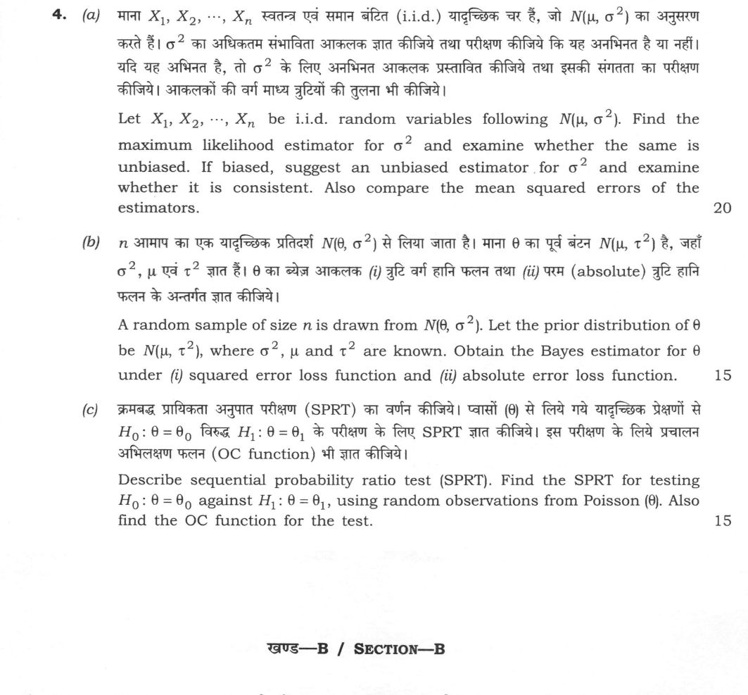
Let X₁, X₂, ⋯, Xₙ be i.i.d. random variables following N(μ, σ²). Find the maximum likelihood estimator for σ² and examine whether the same is unbiased. If biased, suggest an unbiased estimator for σ² and examine whether it is consistent. Also compare the mean squared errors of the estimators. 20 marks
A random sample of size n is drawn from N(θ, σ²). Let the prior distribution of θ be N(μ, τ²), where σ², μ and τ² are known. Obtain the Bayes estimator for θ under (i) squared error loss function and (ii) absolute error loss function. 15 marks
Describe sequential probability ratio test (SPRT). Find the SPRT for testing H₀ : θ = θ₀ against H₁ : θ = θ₁, using random observations from Poisson (θ). Also find the OC function for the test. 15 marks
हिंदी में प्रश्न पढ़ें
माना X₁, X₂, ⋯, Xₙ स्वतन्त्र एवं समान बंटित (i.i.d.) यादृच्छिक चर हैं, जो N(μ, σ²) का अनुसरण करते हैं। σ² का अधिकतम संभाविता आकलक ज्ञात कीजिये तथा परीक्षण कीजिये कि यह अनभिनत है या नहीं। यदि यह अभिनत है, तो σ² के लिये अनभिनत आकलक प्रस्तावित कीजिये तथा इसकी संगता का परीक्षण कीजिये। आकलकों की वर्ग माध्य त्रुटियों की तुलना भी कीजिये। (20 अंक)
n आमाप का एक यादृच्छिक प्रतिदर्श N(θ, σ²) से लिया जाता है। माना θ का पूर्व बंटन N(μ, τ²) है, जहाँ σ², μ एवं τ² ज्ञात हैं। θ का बेयेज आकलक (i) त्रुटि वर्ग हानि फलन तथा (ii) परम (absolute) त्रुटि हानि फलन के अन्तर्गत ज्ञात कीजिये। (15 अंक)
क्रमबद्ध प्रायिकता अनुपात परीक्षण (SPRT) का वर्णन कीजिये। प्वासों (θ) से लिये गये यादृच्छिक प्रेक्षणों से H₀ : θ = θ₀ विरुद्ध H₁ : θ = θ₁ के परीक्षण के लिये SPRT ज्ञात कीजिये। इस परीक्षण के लिये प्रचालन अभिलक्षण फलन (OC function) भी ज्ञात कीजिये। (15 अंक)
Model answer
Drafted with AI by UPSC Answer Check against this question's marking rubric, to the expected length. UPSC does not publish answers for Mains — this is one way to score well, not an official key. How we build rubrics and answers.
(a) MLE of σ², bias, consistency and MSE
MLE of σ². With μ and σ² both unknown, the log-likelihood is
log L = −(n/2) log(2π) − (n/2) log σ² − Σ(Xᵢ − μ)²/(2σ²).
- ∂log L/∂μ = Σ(Xᵢ − μ)/σ² = 0 gives μ̂ = X̄.
- ∂log L/∂σ² = −n/(2σ²) + Σ(Xᵢ − μ)²/(2σ⁴) = 0; substituting μ̂ gives σ̂² = (1/n) Σ(Xᵢ − X̄)².
At (X̄, σ̂²) the Hessian is diagonal with entries −n/σ̂² and −n/(2σ̂⁴), both negative, so this is a maximum. By invariance, the MLE of σ is √σ̂².
Unbiasedness. Write SS = Σ(Xᵢ − X̄)². For a normal sample SS/σ² ~ χ²ₙ₋₁, so E(SS) = (n − 1)σ² and V(SS) = 2(n − 1)σ⁴. Hence
E(σ̂²) = (n − 1)σ²/n ≠ σ², bias = −σ²/n.
The MLE is biased (it under-estimates σ²), though asymptotically unbiased.
Unbiased estimator and its consistency. Correcting the divisor gives
s² = SS/(n − 1), E(s²) = σ².
V(s²) = 2(n − 1)σ⁴/(n − 1)² = 2σ⁴/(n − 1). Since E(s²) = σ² and V(s²) → 0 as n → ∞, Chebyshev's inequality gives P(|s² − σ²| > ε) ≤ 2σ⁴/[(n − 1)ε²] → 0. So s² is consistent for σ². (σ̂² is consistent too, since its bias and variance both vanish.)
Mean squared errors.
- MSE(s²) = V(s²) = 2σ⁴/(n − 1)
- V(σ̂²) = 2(n − 1)σ⁴/n², so MSE(σ̂²) = 2(n − 1)σ⁴/n² + σ⁴/n² = (2n − 1)σ⁴/n²
Then MSE(s²) − MSE(σ̂²) = σ⁴(3n − 1)/[n²(n − 1)] > 0 for every n ≥ 2. The biased MLE has the smaller MSE: its small bias is more than repaid by its lower variance. For example, n = 5 gives 0.36σ⁴ against 0.50σ⁴. More generally, among estimators c·SS the MSE σ⁴[2(n − 1)c² + (c(n − 1) − 1)²] is minimised at c = 1/(n + 1), giving 2σ⁴/(n + 1). Unbiasedness and minimum MSE therefore need not coincide.
| Estimator | Bias | Variance | MSE | Consistent |
|---|---|---|---|---|
| σ̂² = SS/n (MLE) | −σ²/n | 2(n − 1)σ⁴/n² | (2n − 1)σ⁴/n² | Yes |
| s² = SS/(n − 1) | 0 | 2σ⁴/(n − 1) | 2σ⁴/(n − 1) | Yes |
(b) Bayes estimators under a normal prior
Likelihood and prior. Since x̄ is sufficient for θ,
L(θ | x) ∝ exp[−n(θ − x̄)²/(2σ²)], and π(θ) ∝ exp[−(θ − μ)²/(2τ²)].
Posterior. Multiplying and completing the square in θ:
π(θ | x) ∝ exp{−½[(n/σ² + 1/τ²)θ² − 2θ(nx̄/σ² + μ/τ²)]}
So θ | x ~ N(μₙ, σₙ²) (the normal prior is conjugate), with
- Posterior precision: 1/σₙ² = n/σ² + 1/τ², i.e. σₙ² = σ²τ²/(nτ² + σ²)
- Posterior mean: μₙ = (nx̄/σ² + μ/τ²)/(n/σ² + 1/τ²) = (nτ²x̄ + σ²μ)/(nτ² + σ²)
(i) Squared error loss, L(θ, d) = (θ − d)². The posterior expected loss E[(θ − d)² | x] = V(θ | x) + (μₙ − d)² is minimised at d = E(θ | x). The Bayes estimator is the posterior mean:
θ̂_B = (nτ²x̄ + σ²μ)/(nτ² + σ²) = w x̄ + (1 − w)μ, where w = nτ²/(nτ² + σ²).
(ii) Absolute error loss, L(θ, d) = |θ − d|. d ↦ E|θ − d| has derivative P(θ < d | x) − P(θ > d | x), which is zero where the posterior probability is split equally. The Bayes estimator is therefore the posterior median. The normal posterior is symmetric about μₙ, so its median equals its mean:
θ̂_B = μₙ = (nτ²x̄ + σ²μ)/(nτ² + σ²), the same estimator as in (i).
The posterior (Bayes) risk under squared error is the posterior variance σₙ² = σ²τ²/(nτ² + σ²). This is smaller than both σ²/n (the variance of x̄) and τ² (the prior variance), because data and prior information are pooled.
Interpretation. The estimator is a precision-weighted average of the sample mean and the prior mean. As n → ∞ or τ² → ∞ (vague prior), w → 1 and θ̂_B → x̄. As τ² → 0 (confident prior), θ̂_B → μ.
(c) SPRT for the Poisson mean and its OC function
The SPRT. Wald's sequential probability ratio test for H₀: θ = θ₀ against H₁: θ = θ₁ takes observations one at a time. After the m-th observation it computes
λₘ = Πᵢ₌₁ᵐ f(xᵢ, θ₁)/f(xᵢ, θ₀).
With constants B < 1 < A, the rule is:
- accept H₀ if λₘ ≤ B;
- reject H₀ (accept H₁) if λₘ ≥ A;
- continue sampling if B < λₘ < A.
For prescribed risks α and β, Wald's approximations are A ≈ (1 − β)/α and B ≈ β/(1 − α). The test terminates with probability one. Among all tests with the same α and β it minimises the expected sample size under both H₀ and H₁ (Wald–Wolfowitz optimality). Using these approximate boundaries, the actual error probabilities α′ and β′ satisfy α′ + β′ ≤ α + β, so the risks are essentially preserved. In practice log λₘ is accumulated as a running sum of Zᵢ = log[f(xᵢ, θ₁)/f(xᵢ, θ₀)].
SPRT for Poisson(θ) (take θ₁ > θ₀). With f(x, θ) = e^(−θ)θˣ/x! and Sₘ = Σᵢ₌₁ᵐ xᵢ:
λₘ = e^(−m(θ₁ − θ₀)) (θ₁/θ₀)^(Sₘ)
log λₘ = Sₘ log(θ₁/θ₀) − m(θ₁ − θ₀).
Dividing log B < log λₘ < log A by log(θ₁/θ₀) > 0, sampling continues while
[log B + m(θ₁ − θ₀)]/log(θ₁/θ₀) < Sₘ < [log A + m(θ₁ − θ₀)]/log(θ₁/θ₀).
H₀ is accepted when Sₘ falls on or below the lower line and rejected when it reaches the upper line. The boundaries in the (m, Sₘ) plane are two parallel straight lines with common slope s = (θ₁ − θ₀)/log(θ₁/θ₀) and intercepts log B/log(θ₁/θ₀) (negative) and log A/log(θ₁/θ₀).
OC function. L(θ) = P_θ(accept H₀). For each θ, choose h = h(θ) ≠ 0 such that E_θ[(f(X, θ₁)/f(X, θ₀))ʰ] = 1. Wald's approximation is
L(θ) = (Aʰ − 1)/(Aʰ − Bʰ).
For the Poisson case:
E_θ[e^(−h(θ₁ − θ₀))(θ₁/θ₀)^(hX)] = e^(−h(θ₁ − θ₀)) · exp{θ[(θ₁/θ₀)ʰ − 1]} = 1.
This gives θ = h(θ₁ − θ₀)/[(θ₁/θ₀)ʰ − 1]. The OC curve is traced parametrically: let h run over the real line, compute θ(h) and L(θ(h)).
Checks.
- h = 1: θ = (θ₁ − θ₀)/(θ₁/θ₀ − 1) = θ₀, and L = (A − 1)/(A − B) = 1 − α.
- h = −1: θ = θ₁, and L = (A⁻¹ − 1)/(A⁻¹ − B⁻¹) = β.
- h → 0: θ → s = (θ₁ − θ₀)/log(θ₁/θ₀), and L → log A/(log A − log B).
- h → +∞: θ → 0 and L → 1. h → −∞: θ → ∞ and L → 0.
ASN function. Here Z = log[f(X, θ₁)/f(X, θ₀)] = X log(θ₁/θ₀) − (θ₁ − θ₀), so E_θ(Z) = θ log(θ₁/θ₀) − (θ₁ − θ₀). The average sample number is
E_θ(N) ≈ [L(θ) log B + (1 − L(θ)) log A]/[θ log(θ₁/θ₀) − (θ₁ − θ₀)].
At θ₀ and θ₁ this is usually well below the fixed sample size that a Neyman–Pearson test with the same α and β would need, which is the practical attraction of the SPRT. The ASN is largest near θ = s, where the evidence favours neither hypothesis and the path of Sₘ drifts between the two lines.
How this answer will be evaluated
Evaluation rubric
Each sub-part is marked on its own, against the marks and word limit printed on the paper.
- (a) Four linked demands for an i.i.d. N(μ, σ²) sample: derive the MLE of σ², test it for unbiasedness, propose an unbiased alternative and check its consistency, and finally compare the mean squared errors of the two estimators. 20 marks
Must cover
- σ̂²_MLE = (1/n)Σ(Xi − X̄)²
- E(σ̂²_MLE) = (n − 1)σ²/n, bias = −σ²/n
- s² = Σ(Xi − X̄)²/(n − 1), unbiased
- Σ(Xi − X̄)²/σ² ~ χ²_{n−1}; V(s²) = 2σ⁴/(n − 1)
- MSE(σ̂²) = (2n − 1)σ⁴/n² < MSE(s²) = 2σ⁴/(n − 1)
Loses marks
- Deriving σ̂² = (1/n)Σ(Xi − μ)² by treating μ as known — with μ unknown the MLE uses X̄ and the χ²_{n−1} result
- Claiming s² is unbiased AND has smaller MSE — the whole point is that the biased MLE wins on MSE
- Forgetting bias² when computing MSE of the MLE
- Quoting V(s²) = 2σ⁴/n instead of 2σ⁴/(n − 1)
- Confusing consistency with unbiasedness, or asserting consistency without showing the variance tends to zero
Earns more
- Unbiased estimator proposed: s² = Σ(Xi − X̄)²/(n − 1) with E(s²) = σ²
- MSE(σ̂²_MLE) = (2n − 1)σ⁴/n² and MSE(s²) = 2σ⁴/(n − 1)
- Comparison: (2n−1)/n² < 2/(n−1) for all n ≥ 2, so the MLE has the smaller MSE; note cΣ(Xi−X̄)² is MSE-minimised at c = 1/(n+1)
- (b) With X1,...,Xn i.i.d. N(θ, σ²) and conjugate prior θ ~ N(μ, τ²) (σ², μ, τ² all known), derive the posterior and hence the Bayes estimator of θ under (i) squared error loss and (ii) absolute error loss. Both loss functions must be treated. 15 marks
Must cover
- Conjugate normal-normal prior
- Posterior θ | x ~ N(μ_n, σ_n²)
- μ_n = (n τ² x̄ + σ² μ)/(n τ² + σ²) = (n x̄/σ² + μ/τ²)/(n/σ² + 1/τ²)
- σ_n² = σ²τ²/(n τ² + σ²)
- Squared error loss → posterior mean; absolute error loss → posterior median; both equal μ_n by symmetry
Loses marks
- Using the likelihood of a single observation instead of the whole sample, so n never appears in μ_n
- Getting the weights the wrong way round (attaching τ² to μ and σ² to x̄)
- Stating the answer for absolute error loss as the posterior mode or the MLE instead of the posterior median
- Not noticing the symmetry of the normal posterior and leaving (ii) unfinished
- Forgetting that the posterior variance is needed to display the posterior fully
Earns more
- Correct likelihood ∝ exp{−n(θ − x̄)²/2σ²} and prior ∝ exp{−(θ − μ)²/2τ²}, with x̄ noted as sufficient
- (ii) Under absolute error loss the Bayes estimator is the posterior median, which for the symmetric normal posterior equals μ_n — the same estimator
- (c) Three demands: describe Wald's sequential probability ratio test in general; specialise it to H0: θ = θ0 versus H1: θ = θ1 for Poisson(θ) observations; and obtain the operating characteristic (OC) function of that test. 15 marks
Must cover
- Wald's SPRT; A = (1 − β)/α, B = β/(1 − α)
- λ_m = e^{−m(θ1 − θ0)}(θ1/θ0)^{ΣXi}
- Straight-line boundaries for S_m = ΣXi against m
- OC function L(θ) = (A^h − 1)/(A^h − B^h)
- θ = h(θ1 − θ0)/[(θ1/θ0)^h − 1]; L(θ0) = 1 − α, L(θ1) = β
Loses marks
- Inverting the boundaries (accepting H0 when λ_m ≥ A) or writing A = α/(1 − β)
- Treating the SPRT as a fixed-sample test and quoting a Neyman-Pearson critical region
- Errors in the exponent: writing λ_m = e^{−(θ1 − θ0)}(θ1/θ0)^{S_m} without the factor m
- Quoting the OC formula but never deriving h(θ) for the Poisson case
- Confusing the OC function L(θ) = P(accept H0|θ) with the power function or with the ASN function E_θ(N)
Earns more
- Continuation region expressed as two parallel straight-line boundaries in S_m versus m, with slope (θ1 − θ0)/log(θ1/θ0)
- Poisson-specific relation θ = h(θ1 − θ0)/[(θ1/θ0)^h − 1], verified at h = 1 (θ = θ0, L = 1 − α) and h = −1 (θ = θ1, L = β)
What "Examine" is asking you to do
Test the proposition the question puts to you and return a finding on how far it holds. Examine stems carry a claim, or ask whether something has happened, and expect evidence weighed both ways before the extent is stated — often with remedial measures attached.
Structure that answers it
Restate the claim as the question frames it → evidence that supports it → evidence that undercuts it → the conditions under which it holds → verdict on how far it stands
Where marks are lost
Stopping at description. An examination has to reach a finding, and “examine with justification” means the extent must be stated, not implied.
Practice this exact question
Write your answer and it is marked point by point against the model answer above — what you covered, what you missed, what you got wrong.
Evaluate my answer →More from Statistics 2026 Paper I
- Q1 (a) (i) Show that for n events A₁, A₂, ⋯, Aₙ P( ⋂_{i=1}^{n} Aᵢ ) ≥ Σ_{i=1}^{n} P(Aᵢ) − (n…
- Q2 (a) (i) Find the moment generating function (m.g.f.) of a random variable X with probabil…
- Q3 (a) Let the joint probability density function of X and Y be f(x, y) = 3/4 ( xy + x²/2 )…
- Q4 (a) Let X₁, X₂, ⋯, Xₙ be i.i.d. random variables following N(μ, σ²). Find the maximum lik…
- Q5 (a) Let Y₁, Y₂, ⋯, Yₙ be n independent observations from a population with mean μ and var…
- Q6 (a) Let l′β be any estimable linear function of parameters β₁, β₂, ⋯, β_p. Then prove tha…
- Q7 The following data are from a two-factor random effects model : | Factor B \ Factor A | B…