Paper II — Q1
(a) Suppose that a given individual in a population has a survival time which is exponential with a hazard rate θ. Each…
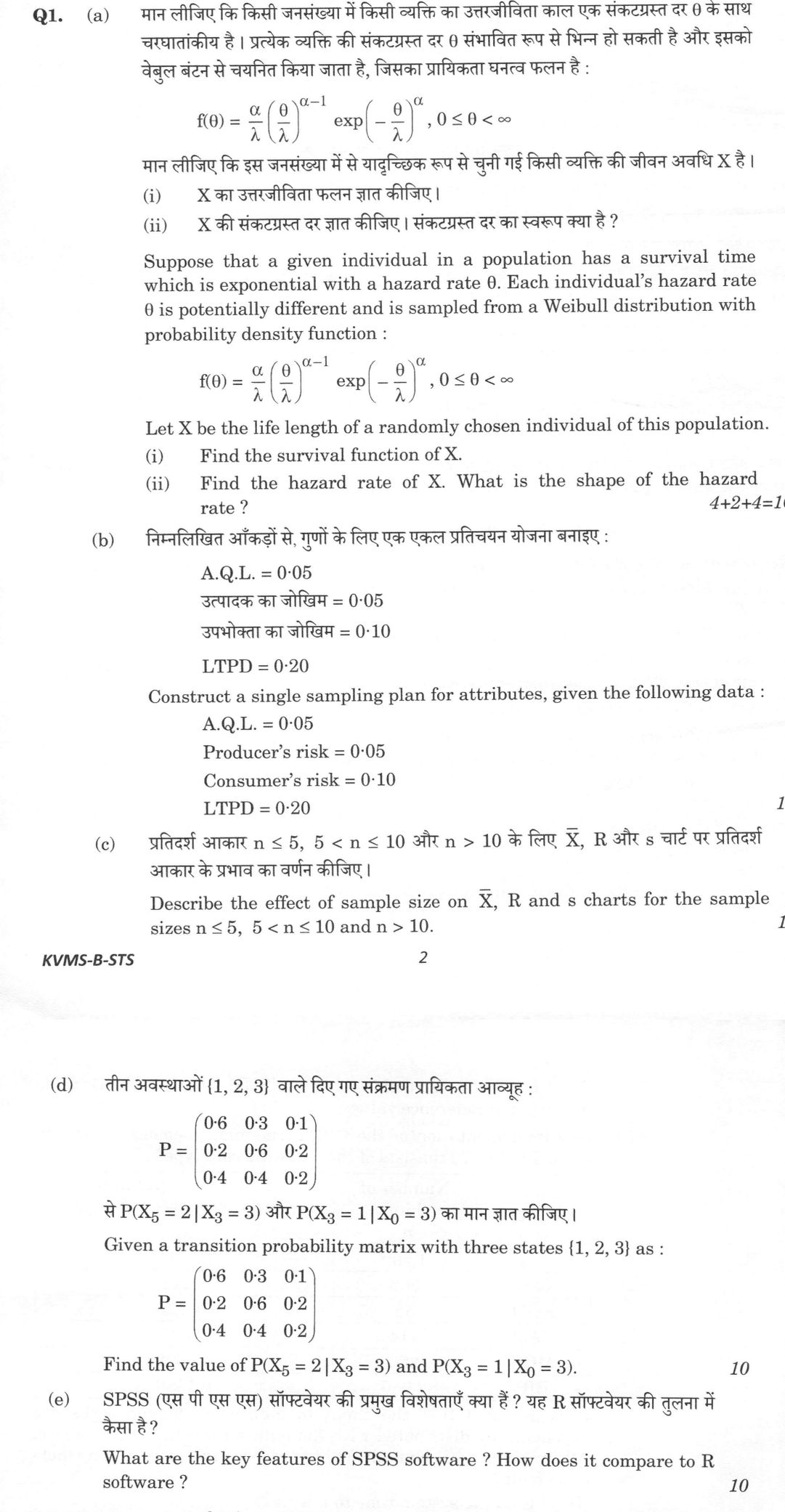
Suppose that a given individual in a population has a survival time which is exponential with a hazard rate θ. Each individual's hazard rate θ is potentially different and is sampled from a Weibull distribution with probability density function :
f(θ) = (α/λ) (θ/λ)^(α−1) exp(−(θ/λ)^α), 0 ≤ θ < ∞
Let X be the life length of a randomly chosen individual of this population. Find the survival function of X.
Find the hazard rate of X. What is the shape of the hazard rate ? 10 marks
Construct a single sampling plan for attributes, given the following data :
A.Q.L. = 0·05 Producer's risk = 0·05 Consumer's risk = 0·10
LTPD = 0·20 10 marks
Describe the effect of sample size on X̄, R and s charts for the sample sizes n ≤ 5, 5 < n ≤ 10 and n > 10. 10 marks
Given a transition probability matrix with three states {1, 2, 3} as :
P = ( 0·6 0·3 0·1 0·2 0·6 0·2 0·4 0·4 0·2 )
Find the value of P(X5 = 2 | X3 = 3) and P(X3 = 1 | X0 = 3). 10 marks
What are the key features of SPSS software ? How does it compare to R software ? 10 marks
हिंदी में प्रश्न पढ़ें
मान लीजिए कि किसी जनसंख्या में किसी व्यक्ति का उत्तरजीविता काल एक संकटप्रस्त दर θ के साथ चरघातांकी है। प्रत्येक व्यक्ति की संकटप्रस्त दर θ संभावित रूप से भिन्न हो सकती है और इसको वेबुल बंटन से चयनित किया जाता है, जिसका प्रायिकता घनत्व फलन है :
f(θ) = (α/λ) (θ/λ)^(α−1) exp(−(θ/λ)^α), 0 ≤ θ < ∞
मान लीजिए कि इस जनसंख्या में से यादृच्छिक रूप से चुनी गई किसी व्यक्ति की जीवन अवधि X है। X का उत्तरजीविता फलन ज्ञात कीजिए।
X की संकटप्रस्त दर ज्ञात कीजिए। संकटप्रस्त दर का स्वरूप क्या है? (10 अंक)
निम्नलिखित आँकड़ों से, गुणों के लिए एक एकल प्रतिचयन योजना बनाइए :
A.Q.L. = 0·05 उत्पादक का जोखिम = 0·05 उपभोक्ता का जोखिम = 0·10
LTPD = 0·20 (10 अंक)
प्रतिदर्श आकार n ≤ 5, 5 < n ≤ 10 और n > 10 के लिए X̄, R और s चार्ट पर प्रतिदर्श आकार के प्रभाव का वर्णन कीजिए। (10 अंक)
तीन अवस्थाओं {1, 2, 3} वाले दिए गए संक्रमण प्रायिकता आव्यूह :
P = ( 0·6 0·3 0·1 0·2 0·6 0·2 0·4 0·4 0·2 )
से P(X5 = 2 | X3 = 3) और P(X3 = 1 | X0 = 3) का मान ज्ञात कीजिए। (10 अंक)
SPSS (एस पी एस एस) सॉफ्टवेयर की प्रमुख विशेषताएँ क्या हैं ? यह R सॉफ्टवेयर की तुलना में कैसा है ? (10 अंक)
Model answer
Drafted with AI by UPSC Answer Check against this question's marking rubric, to the expected length. UPSC does not publish answers for Mains — this is one way to score well, not an official key. How we build rubrics and answers.
(a) Exponential lifetime with Weibull-distributed hazard (frailty mixture)
(i) Given θ, X is exponential: S(x | θ) = P(X > x | θ) = e^(−θx). Averaging over the Weibull law of θ, S_X(x) = E_θ[e^(−θx)] = ∫₀^∞ e^(−θx) (α/λ)(θ/λ)^(α−1) e^(−(θ/λ)^α) dθ = ∫₀^∞ e^(−λx u^(1/α)) e^(−u) du (u = (θ/λ)^α), i.e. the Laplace transform of the Weibull(α, λ) density evaluated at x. For general α it has no elementary closed form. For α = 1 (θ exponential with mean λ), S_X(x) = 1/(1 + λx), a Lomax (Pareto type II) law.
(ii) f_X(x) = −S_X′(x) = E[θe^(−θx)], so h_X(x) = f_X(x)/S_X(x) = E[θe^(−θx)]/E[e^(−θx)] = E[θ | X > x], the mean hazard among those still alive at x. Differentiating, h_X′(x) = −E[θ²e^(−θx)]/E[e^(−θx)] − (E[θe^(−θx)]/E[e^(−θx)])² = −Var(θ | X > x) < 0. The hazard of X is strictly decreasing (DFR), from h_X(0) = E(θ) = λΓ(1 + 1/α) towards 0: high-risk individuals fail early, so the surviving population is increasingly made of low-θ individuals, although each individual has a constant hazard. For α = 1, h_X(x) = λ/(1 + λx). (Check for α = 2, λ = 1: h(0) = 0.886, h(1) = 0.701, h(5) = 0.335.)
(b) Single sampling plan for attributes
p₁ = AQL = 0.05 with Pₐ = 1 − α = 0.95; p₂ = LTPD = 0.20 with Pₐ = β = 0.10. With the Poisson approximation the plan (n, c) must satisfy Σ_d=0^c e^(−np₁)(np₁)^d/d! = 0.95 and Σ_d=0^c e^(−np₂)(np₂)^d/d! = 0.10. Operating ratio R = p₂/p₁ = 0.20/0.05 = 4.0. From Cameron's table of unity values, c = 4 gives np₁ = 1.970 and np₂ = 7.994, ratio 4.058 (closest to 4; c = 5 gives 3.55, c = 3 gives 4.89). n = np₁/p₁ = 1.970/0.05 = 39.4 and n = np₂/p₂ = 7.994/0.20 = 39.97, so take n = 40, c = 4: inspect 40 items, accept the lot if 4 or fewer are defective, reject if 5 or more. Check (Poisson): at p = 0.05, np = 2, Pₐ = 0.947 (α ≈ 0.053); at p = 0.20, np = 8, Pₐ = 0.0996 (β ≈ 0.100). With n = 39, β would be 0.112 > 0.10, so n = 40 is needed.
(c) Effect of subgroup size on X̄, R and s charts
X̄ chart: limits X̿ ± 3σ/√n (= X̿ ± A₂R̄ or X̿ ± A₃s̄) narrow as 1/√n, so larger subgroups detect smaller shifts in the mean faster, at higher sampling cost; σ is estimated by R̄/d₂ or s̄/c₄.
n ≤ 5: the R chart is recommended. The range is almost as efficient as s (relative efficiency 1.000, 0.992, 0.975, 0.955 for n = 2, 3, 4, 5) and simple to compute. D₃ = 0 (for n ≤ 6) and B₃ = 0 (for n ≤ 5), so the dispersion charts have no lower control limit.
5 < n ≤ 10: the efficiency of R falls (0.930 at n = 6, about 0.85 at n = 10) because it uses only the two extreme values; the s chart is preferable, though R is still acceptable. Positive LCLs appear (B₃ = 0.030 at n = 6, D₃ = 0.076 at n = 7), so decreases in variability can also be detected.
n > 10: the range becomes inefficient and the s chart (limits B₃s̄, B₄s̄) with the X̄ chart based on A₃s̄ should be used. Very large n makes the X̄ limits so tight that trivial shifts signal and makes rational subgrouping harder.
(d) Multi-step transition probabilities
The chain is time-homogeneous, so by the Chapman-Kolmogorov equations P(Xₘ₊ₖ = j | Xₘ = i) = p_ij^(k), the (i, j) entry of P^k. Row 3 of P²: p₃₁^(2) = 0.4(0.6) + 0.4(0.2) + 0.2(0.4) = 0.40; p₃₂^(2) = 0.4(0.3) + 0.4(0.6) + 0.2(0.4) = 0.44; p₃₃^(2) = 0.4(0.1) + 0.4(0.2) + 0.2(0.2) = 0.16 (sum 1). P(X₅ = 2 | X₃ = 3) = p₃₂^(2) = 0.44. p₃₁^(3) = Σₖ p₃ₖ^(2) p_k1 = 0.40(0.6) + 0.44(0.2) + 0.16(0.4) = 0.240 + 0.088 + 0.064. P(X₃ = 1 | X₀ = 3) = p₃₁^(3) = 0.392.
(e) SPSS: key features and comparison with R
IBM SPSS Statistics is a proprietary, menu-driven statistical package. Key features: a spreadsheet-like Data Editor with Data View and Variable View (variable and value labels, user-defined missing values, measurement levels); strong data management (Recode, Compute, Select Cases, Split File, Aggregate, Merge, Weight) and import from Excel, CSV, SAS, Stata and databases; wide procedure coverage (descriptives, crosstabs and χ², t-tests, ANOVA/GLM, regression including logistic, factor, cluster and discriminant analysis, reliability, non-parametric tests, time series, survival), with add-on modules such as Advanced Statistics, Custom Tables, Complex Samples and AMOS for structural equation models; an Output Viewer with editable pivot tables and charts exportable to Word, Excel and PDF; and Command Syntax with a Paste button that turns menu actions into re-runnable scripts, plus Python and R extensions.
Comparison with R: R is free, open-source (GPL) and script-based; SPSS needs a paid licence and is GUI-based, so SPSS is quicker to learn while R has a steeper learning curve but far more flexibility. R's CRAN repository (over 20,000 packages) makes new methods available much sooner, and its graphics (e.g. ggplot2) are more flexible; R, with RStudio and R Markdown, is the norm for simulation, custom modelling and reproducible research. SPSS handles labelled survey data, missing-value codes and complex-survey weighting natively, gives formatted output without programming, and offers vendor support, which is why it remains common in social-science and survey offices; R keeps its data in memory by default, which can limit very large files. The two are complementary.
How this answer will be evaluated
Evaluation rubric
Each sub-part is marked on its own, against the marks and word limit printed on the paper.
- (a) A frailty/mixture problem: X | theta ~ Exponential(hazard theta) and theta ~ Weibull(shape alpha, scale lambda) with pdf f(theta) = (alpha/lambda)(theta/lambda)^(alpha-1) exp(-(theta/lambda)^alpha). Candidate must (i) derive the unconditional survival function S_X(x) by mixing (un-conditioning) over theta, and (ii) obtain the unconditional hazard rate h_X(x) and state its shape. Both sub-parts must be answered. 10 marks
Must cover
- S(x | theta) = exp(-theta x)
- S_X(x) = E_theta[exp(-theta x)] (Laplace transform of the frailty distribution)
- h_X(x) = E[theta | X > x]
- h_X'(x) = -Var(theta | X > x) < 0
- Decreasing hazard rate (DFR) / decreasing failure rate
- h_X(0) = lambda*Gamma(1 + 1/alpha)
- alpha = 1 case: S_X(x) = 1/(1 + lambda x), Lomax/Pareto
Loses marks
- Writing S_X(x) = exp(-(x/lambda)^alpha), i.e. confusing the mixing distribution of theta with the distribution of X - this is the single commonest error and earns no marks for part (i)
- Claiming the hazard of X is constant (theta) because each individual is exponential - the population hazard is NOT the average of individual hazards
- Attempting a closed-form integral for general alpha and producing a fabricated Gamma-function expression
- Giving only S_X(x) and stopping, without deriving h(x) = f(x)/S(x) or commenting on its shape as the question explicitly demands
- Stating the hazard is 'bathtub' or 'increasing' - any mixture of exponentials is necessarily DFR
Earns more
- States h_X(0) = E(theta) = lambda*Gamma(1 + 1/alpha) and h_X(x) -> 0 as x -> infinity
- Notes the general-alpha integral has no elementary closed form, and gives the alpha = 1 special case S_X(x) = 1/(1 + lambda x), h_X(x) = lambda/(1 + lambda x) (Lomax/Pareto)
- (b) Design a single sampling plan by attributes, i.e. find the sample size n and acceptance number c, given AQL p1 = 0.05 with producer's risk alpha = 0.05 and LTPD p2 = 0.20 with consumer's risk beta = 0.10. The plan must be stated explicitly and its two risk conditions verified. 10 marks
Must cover
- AQL p1 = 0.05, LTPD p2 = 0.20, alpha = 0.05, beta = 0.10
- Operating ratio R = p2/p1 = 4.0
- Cameron's table of Poisson unity values (np1 for P = 0.95, np2 for P = 0.10)
- c = 4
- n = 40
- Plan: sample 40, accept if defectives <= 4
- Verification alpha ~ 0.053, beta ~ 0.0996
Loses marks
- Inverting the ratio (computing p1/p2 = 0.25) and reading the wrong row of Cameron's table
- Picking c = 3 or c = 5 without comparing |R_table - 4.0|; c = 5 (R = 3.549) is much further from 4.0 than c = 4 (R = 4.057)
- Computing n from np1 but then not rounding consistently, giving n = 39 - which leaves beta = 0.112 > 0.10, violating the consumer's risk; n = 40 is the correct rounding
- Forgetting to state the actual decision rule (sample size AND acceptance number AND accept/reject action)
- Using the hypergeometric distribution: the lot size is not given, so the Poisson (or binomial) approximation is what is expected
Earns more
- States the two design conditions P_a(p1 = 0.05) = 1 - alpha = 0.95 and P_a(p2 = 0.20) = beta = 0.10, with the Poisson (or binomial) form of P_a
- States the operating rule (sample 40, accept if d <= 4, reject if d >= 5) and verifies actual risks alpha ~ 0.053, beta ~ 0.0996
- (c) Describe how the choice of subgroup size n affects the X-bar, R and s control charts, treating the three stated ranges separately: n <= 5, 5 < n <= 10, and n > 10. The answer must cover both which dispersion chart is appropriate in each range and what happens to the limits and sensitivity of the X-bar chart. 10 marks
Must cover
- A2, A3, d2, c4, D3, D4, B3, B4 control-chart constants
- sigma-hat = R-bar/d2 and sigma-hat = s-bar/c4
- Relative efficiency of range versus standard deviation falls with n (about 0.955 at n = 5, 0.850 at n = 10)
- R chart for n <= 5, s chart for n > 10
- X-bar limit half-width = 3 sigma/sqrt(n)
- D3 = 0 for n <= 6, B3 = 0 for n <= 5
Loses marks
- Answering only about the X-bar chart and ignoring how n decides between R and s, which is the core of the question
- Asserting that the R chart is 'always inferior' - for n <= 5 it is over 95 per cent as efficient as the s chart and is the standard recommendation
- Confusing the sample sigma s with sigma-hat: forgetting the c4 unbiasing divisor when estimating sigma from s-bar
- Saying the control limits widen as n increases (they narrow, as 1/sqrt(n))
- Not treating the three stated ranges separately - the question explicitly names n <= 5, 5 < n <= 10 and n > 10
Earns more
- 5 < n <= 10: efficiency of R drops (0.930 at n = 6, about 0.850 at n = 10); s chart becomes preferable though R is still acceptable
- Notes the LCL behaviour: D3 = 0 for n <= 6 and B3 = 0 for n <= 5, so no effective lower control limit exists for small subgroups; positive LCLs appear from n = 7 (R) and n = 6 (s)
- (d) For the given 3-state transition probability matrix P, use the Chapman-Kolmogorov equations (time-homogeneity) to evaluate the two-step probability P(X5 = 2 | X3 = 3) = p_32^(2) and the three-step probability P(X3 = 1 | X0 = 3) = p_31^(3). Both values must be computed. 10 marks
Must cover
- Chapman-Kolmogorov equation p_ij^(m+n) = sum_k p_ik^(m) p_kj^(n)
- Time-homogeneous Markov chain
- Third row of P^2 = (0.40, 0.44, 0.16)
- P(X5 = 2 | X3 = 3) = 0.44
- P(X3 = 1 | X0 = 3) = 0.392
Loses marks
- Computing P^5 instead of P^2 for the first part - the gap is 5 - 3 = 2 steps, and homogeneity makes only the gap matter
- Reading the wrong entry: taking column 3, row 2 (p_23) instead of row 3, column 2 (p_32)
- Arithmetic slips in matrix multiplication - failing to check that each row of P^2 sums to 1 (0.46 + 0.40 + 0.14 = 1, etc.)
- Confusing state labels with matrix indices when the states are named {1, 2, 3}
- Using the stationary distribution instead of the n-step transition probabilities
Earns more
- Correctly computes the third row of P^2 as (0.40, 0.44, 0.16)
- States P(X3 = 1 | X0 = 3) = 0.392, and checks that the rows of P^2 / P^3 sum to 1
- (e) Two parts: (i) list and explain the key features of IBM SPSS Statistics, and (ii) compare SPSS with R on the dimensions that matter to a statistician - cost/licensing, interface, extensibility, output, graphics, data handling and suitability for different tasks. Both parts must be answered. 10 marks
Must cover
- IBM SPSS Statistics (Statistical Package for the Social Sciences)
- Data View / Variable View, variable and value labels, defined missing values
- SPSS Command Syntax and the Paste button; Output Viewer pivot tables
- Modules: Advanced Statistics, Custom Tables, Complex Samples, AMOS
- R is free open-source (GPL); CRAN; ggplot2; RStudio / R Markdown
- Proprietary licence versus open source; GUI versus script
Loses marks
- Writing a generic 'software is useful' essay without naming a single SPSS-specific feature such as the Variable View, the Paste-syntax facility or a named module
- Answering only part (i) and omitting the explicit comparison with R that the question demands
- Claiming R 'cannot do' a named analysis or that SPSS 'has no programming language' - SPSS has Command Syntax plus Python and R plug-ins
- One-sided advocacy: a balanced answer must concede SPSS's advantages (labelled data, complex-survey module, ready-formatted output, vendor validation) as well as R's
- Confusing SPSS with SAS or with SPSS Modeler and attributing the wrong features
Earns more
- Lists SPSS's analytical coverage and modules (descriptives, crosstabs, t-test, ANOVA/GLM, regression, factor analysis, cluster, reliability, non-parametric, survival; Advanced Statistics, Custom Tables, Complex Samples, AMOS, Modeler)
- Explains the Output Viewer with editable pivot tables and charts, and the SPSS Command Syntax / Paste facility that makes GUI work reproducible and scriptable
What "Solve" is asking you to do
Choose the method, then carry it through to a final answer. Identifying what kind of problem this is and why that method applies is the first thing marked; a correct figure arrived at invisibly earns almost nothing.
Structure that answers it
Given data and what is required → method chosen, with the reason it applies → set-up (equation, circuit, free body, trial balance) → working, step by step → answer with units and any condition of validity
Where marks are lost
Doing the middle steps mentally and writing only the result. In mathematics papers, a further loss comes from giving a decimal where the exact value in surds or fractions was wanted, or from skipping the justification a part explicitly asks for.
Practice this exact question
Write your answer and it is marked point by point against the model answer above — what you covered, what you missed, what you got wrong.
Evaluate my answer →More from Statistics 2026 Paper II
- Q1 (a) Suppose that a given individual in a population has a survival time which is exponent…
- Q2 (a) (i) Describe the construction of a CUSUM chart with Decision interval and Reference v…
- Q3 (a) How will you draw the OC curve for a single sampling plan with sample size 5, if the…
- Q4 (a) (i) Discuss the theoretical basis of the sequential probability ratio test (SPRT) in…