Paper II — Q4
(a) (i) Discuss the theoretical basis of the sequential probability ratio test (SPRT) in acceptance sampling. Explain how…
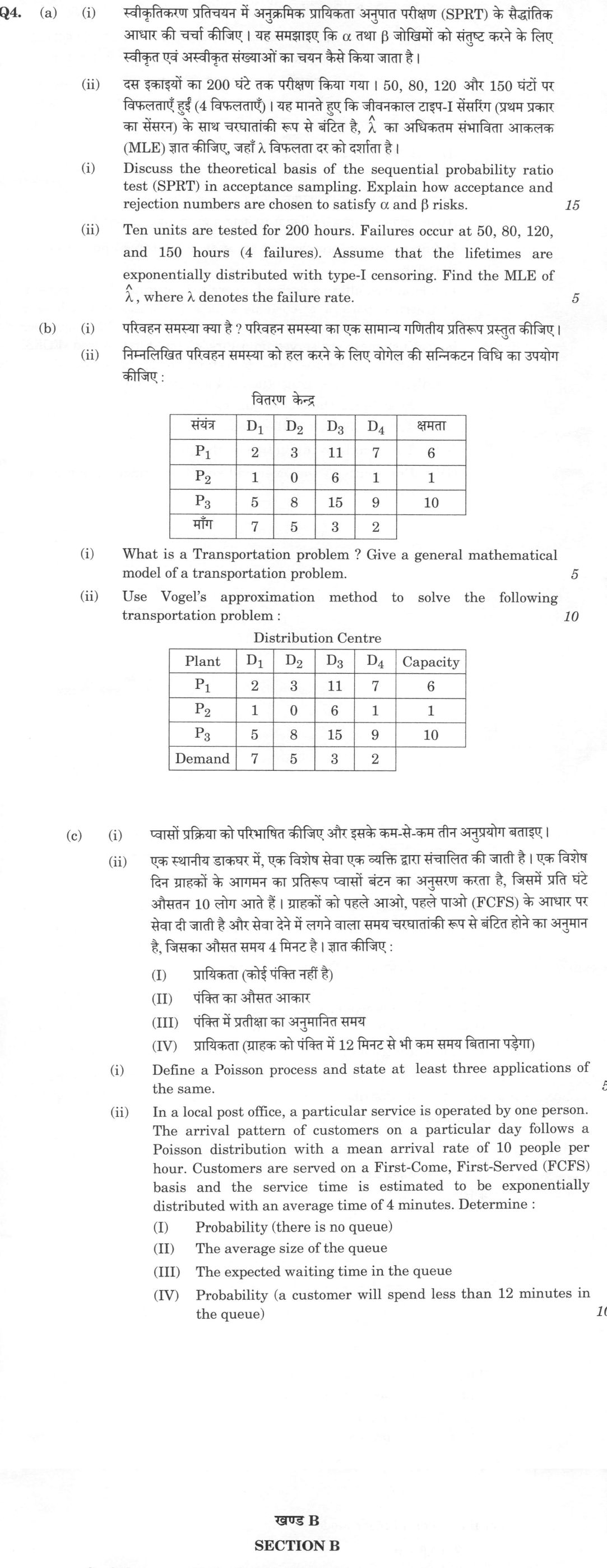
Discuss the theoretical basis of the sequential probability ratio test (SPRT) in acceptance sampling. Explain how acceptance and rejection numbers are chosen to satisfy α and β risks. 15 marks
Ten units are tested for 200 hours. Failures occur at 50, 80, 120, and 150 hours (4 failures). Assume that the lifetimes are exponentially distributed with type-I censoring. Find the MLE of λ̂, where λ denotes the failure rate. 5 marks
What is a Transportation problem ? Give a general mathematical model of a transportation problem. 5 marks
Use Vogel’s approximation method to solve the following transportation problem : Distribution Centre Plant D₁ D₂ D₃ D₄ Capacity P₁ 2 3 11 7 6 P₂ 1 0 6 1 1 P₃ 5 8 15 9 10 Demand 7 5 3 2 10 marks
Define a Poisson process and state at least three applications of the same. 5 marks
In a local post office, a particular service is operated by one person. The arrival pattern of customers on a particular day follows a Poisson distribution with a mean arrival rate of 10 people per hour. Customers are served on a First-Come, First-Served (FCFS) basis and the service time is estimated to be exponentially distributed with an average time of 4 minutes. Determine : (I) Probability (there is no queue) (II) The average size of the queue (III) The expected waiting time in the queue (IV) Probability (a customer will spend less than 12 minutes in the queue) 10 marks
हिंदी में प्रश्न पढ़ें
स्वीकृतिकरण प्रतिचयन में अनुक्रमिक प्रायिकता अनुपात परीक्षण (SPRT) के सैद्धांतिक आधार की चर्चा कीजिए। यह समझाइए कि α तथा β जोखिमों को संतुष्ट करने के लिए स्वीकृत एवं अस्वीकृत संख्याओं का चयन कैसे किया जाता है। (15 अंक)
दस इकाइयों का 200 घंटे तक परीक्षण किया गया। 50, 80, 120 और 150 घंटों पर विफलताएँ हुईं (4 विफलताएँ)। यह मानते हुए कि जीवनकाल टाइप-I सेंसरिंग (प्रथम प्रकार का सेंसर) के साथ चरघातांकी रूप से बंटित है, λ̂ का अधिकतम संभाविता आकलक (MLE) ज्ञात कीजिए, जहाँ λ विफलता दर को दर्शाता है। (5 अंक)
परिवहन समस्या क्या है ? परिवहन समस्या का एक सामान्य गणितीय प्रतिरूप प्रस्तुत कीजिए। (5 अंक)
निम्नलिखित परिवहन समस्या को हल करने के लिए वोगेल की सन्निकटन विधि का उपयोग कीजिए : वितरण केन्द्र संयंत्र D₁ D₂ D₃ D₄ क्षमता P₁ 2 3 11 7 6 P₂ 1 0 6 1 1 P₃ 5 8 15 9 10 माँग 7 5 3 2 (10 अंक)
प्वासों प्रक्रिया को परिभाषित कीजिए और इसके कम-से-कम तीन अनुप्रयोग बताइए । (5 अंक)
एक स्थानीय डाकघर में, एक विशेष सेवा एक व्यक्ति द्वारा संचालित की जाती है । एक विशेष दिन ग्राहकों के आगमन का प्रतिरूप प्वासों बंटन का अनुसरण करता है, जिसमें प्रति घंटे औसतन 10 लोग आते हैं । ग्राहकों को पहले आओ, पहले पाओ (FCFS) के आधार पर सेवा दी जाती है और सेवा देने में लगने वाला समय चरघातांकी रूप से बंटित होने का अनुमान है, जिसका औसत समय 4 मिनट है । ज्ञात कीजिए : (I) प्रायिकता (कोई पंक्ति नहीं है) (II) पंक्ति का औसत आकार (III) पंक्ति में प्रतीक्षा का अनुमानित समय (IV) प्रायिकता (ग्राहक को पंक्ति में 12 मिनट से भी कम समय बिताना पड़ेगा) (10 अंक)
Model answer
Drafted with AI by UPSC Answer Check against this question's marking rubric, to the expected length. UPSC does not publish answers for Mains — this is one way to score well, not an official key. How we build rubrics and answers.
(a) (i) SPRT in acceptance sampling
Wald's sequential probability ratio test treats lot acceptance as a test of H₀: p = p₁ (AQL) against H₁: p = p₂ (LTPD), p₂ > p₁, with producer's risk α = P(reject | p₁) and consumer's risk β = P(accept | p₂). Items are inspected one at a time; after n items containing d defectives the likelihood ratio is λₙ = [p₂^d (1 − p₂)^(n−d)] / [p₁^d (1 − p₁)^(n−d)]. Rule: accept the lot if λₙ ≤ B, reject if λₙ ≥ A, otherwise inspect one more item, with Wald's approximations A = (1 − β)/α and B = β/(1 − α). (These ignore the overshoot of the boundaries; the achieved risks satisfy α′ + β′ ≤ α + β.)
Taking logarithms, with k = ln[p₂(1 − p₁)/p₁(1 − p₂)], the continuation region becomes the band between two parallel lines in the (n, d) plane: acceptance line d = sn − h₁, rejection line d = sn + h₂, where s = ln[(1 − p₁)/(1 − p₂)]/k, h₁ = ln[(1 − α)/β]/k, h₂ = ln[(1 − β)/α]/k. At stage n the acceptance number is aₙ = the largest integer ≤ sn − h₁ and the rejection number is rₙ = the smallest integer ≥ sn + h₂; accept if d ≤ aₙ, reject if d ≥ rₙ, continue otherwise. The slope s (between p₁ and p₂) depends only on the two quality levels, while α and β enter only through the intercepts h₁ and h₂, which is how the two risks are enforced; no acceptance is possible before n > h₁/s. The OC function is L(p) = (Aʰ − 1)/(Aʰ − Bʰ), giving L(p₁) = 1 − α and L(p₂) = β, and the ASN is E(n | p) ≈ [L(p) ln B + (1 − L(p)) ln A]/E(z). By the Wald-Wolfowitz theorem the SPRT minimises the expected sample number at both p₁ and p₂ among all plans with the same α and β (often about half the single-sampling n); in practice the plan is truncated at some n₀.
(a) (ii) MLE of λ under type-I censoring
n = 10 units, test stopped at T₀ = 200 h, r = 4 failures at 50, 80, 120, 150 h and 6 survivors. L(λ) = Πᵢ₌₁⁴ λe^(−λtᵢ) × [e^(−200λ)]⁶ = λ⁴ e^(−λT), T = Σtᵢ + (n − r)T₀. ln L = 4 ln λ − λT; d ln L/dλ = 4/λ − T = 0 gives λ̂ = r/T (second derivative −4/λ² < 0). Total time on test T = (50 + 80 + 120 + 150) + 6 × 200 = 400 + 1200 = 1600 unit-hours. λ̂ = 4/1600 = 0.0025 failures per hour (estimated MTTF = 1/λ̂ = 400 hours).
(b) (i) Transportation problem and its model
A transportation problem is a special linear programming problem of shipping a single commodity from m sources (supplies aᵢ) to n destinations (demands bⱼ) at minimum total cost, cᵢⱼ being the cost per unit from source i to destination j and xᵢⱼ the quantity shipped. Minimise Z = Σᵢ₌₁ᵐ Σⱼ₌₁ⁿ cᵢⱼ xᵢⱼ subject to Σⱼ xᵢⱼ = aᵢ (i = 1, …, m), Σᵢ xᵢⱼ = bⱼ (j = 1, …, n), xᵢⱼ ≥ 0. A feasible solution exists when the problem is balanced, Σaᵢ = Σbⱼ; otherwise a dummy source or destination with zero costs is added. Only m + n − 1 constraints are independent, so a basic feasible solution has m + n − 1 occupied cells.
(b) (ii) Vogel's approximation method and optimality
Supply 6 + 1 + 10 = 17 = demand 7 + 5 + 3 + 2, so the problem is balanced; m + n − 1 = 6. Step 1: row penalties (difference of the two lowest costs) 1, 1, 3; column penalties 1, 3, 5, 6. Largest is 6 (D₄); its least cost is 1 at P₂: x₂₄ = 1, P₂ exhausted. Step 2: row penalties P₁ 1, P₃ 3; column penalties 3, 5, 4, 2. Largest 5 (D₂): least cost 3 at P₁: x₁₂ = 5, D₂ satisfied, P₁ has 1 left. Step 3: row penalties P₁ 5, P₃ 4; column penalties 3, 4, 2. Largest 5 (P₁): least cost 2 at D₁: x₁₁ = 1, P₁ exhausted. Step 4: only P₃ remains: x₃₁ = 6, x₃₃ = 3, x₃₄ = 1. VAM solution (6 cells, non-degenerate): x₁₁ = 1, x₁₂ = 5, x₂₄ = 1, x₃₁ = 6, x₃₃ = 3, x₃₄ = 1; cost = 2 + 15 + 1 + 30 + 45 + 9 = ₹102.
MODI test (cᵢⱼ = uᵢ + vⱼ on occupied cells, u₁ = 0): v₁ = 2, v₂ = 3, u₃ = 3, v₃ = 12, v₄ = 6, u₂ = −5. Opportunity costs dᵢⱼ = cᵢⱼ − uᵢ − vⱼ: d₁₃ = −1, d₂₃ = −1, d₁₄ = 1, d₂₁ = 4, d₂₂ = 2, d₃₂ = 2. Negative values, so the VAM solution is not optimal. Enter (1,3): loop (1,3)+ (3,3)− (3,1)+ (1,1)−, θ = 1, cost ₹101. Enter (2,3): loop (2,3)+ (3,3)− (3,4)+ (2,4)−, θ = 1, cost ₹100. Re-test (u₁ = 0): v₂ = 3, v₃ = 11, u₂ = −5, u₃ = 4, v₁ = 1, v₄ = 5; all dᵢⱼ ≥ 0, so the solution is optimal. Optimal: x₁₂ = 5, x₁₃ = 1, x₂₃ = 1, x₃₁ = 7, x₃₃ = 1, x₃₄ = 2; minimum cost ₹100 (the VAM starting solution cost ₹102).
(c) (i) Poisson process and applications
A counting process N(t), t ≥ 0 is a Poisson process with rate λ if N(0) = 0, its increments over disjoint intervals are independent and stationary, and it is orderly: P[N(h) = 1] = λh + o(h), P[N(h) ≥ 2] = o(h). Then P[N(t) = n] = e^(−λt)(λt)ⁿ/n!, n = 0, 1, 2, …, with E[N(t)] = V[N(t)] = λt; equivalently the inter-arrival times are independent exponential with mean 1/λ. Applications: arrivals of customers or calls in queueing systems; emissions in radioactive decay; failures of components in reliability studies; insurance claims or road accidents over time; defects per unit length or area (basis of the c chart).
(c) (ii) M/M/1 queue at the post office
λ = 10 per hour, μ = 60/4 = 15 per hour, ρ = λ/μ = 2/3 < 1. (I) Server idle (nobody in the system): P₀ = 1 − ρ = 1/3 ≈ 0.333. Read strictly as "nobody waiting", P(N ≤ 1) = 1 − ρ² = 5/9 ≈ 0.556. (II) L_q = ρ²/(1 − ρ) = (4/9)/(1/3) = 4/3 ≈ 1.33 customers (Lₛ = ρ/(1 − ρ) = 2). (III) W_q = L_q/λ = (4/3)/10 = 2/15 hour = 8 minutes (Wₛ = 1/(μ − λ) = 12 minutes). (IV) The waiting time in the queue has P(W_q = 0) = 1 − ρ and P(W_q > t) = ρe^(−(μ−λ)t). With t = 12 min = 0.2 h and μ − λ = 5 per hour: P(W_q > 0.2) = (2/3)e^(−1) = 0.245, so P(W_q < 12 minutes) = 1 − (2/3)e^(−1) ≈ 0.755. (If the time spent in the whole system is meant, P(Wₛ < 0.2) = 1 − e^(−1) ≈ 0.632.)
How this answer will be evaluated
Evaluation rubric
Each sub-part is marked on its own, against the marks and word limit printed on the paper.
- (a)(i) Two linked demands: (i) set out the theoretical basis of Wald's sequential probability ratio test as applied to acceptance sampling by attributes, and (ii) explain precisely how the acceptance and rejection numbers (the two boundary lines) are determined so that the producer's risk alpha and consumer's risk beta are met. 15 marks
Must cover
- Wald's sequential probability ratio test (SPRT), 1943-47
- H0: p = p1 (AQL), H1: p = p2 (LTPD)
- A = (1 - beta)/alpha, B = beta/(1 - alpha)
- Acceptance line d = s n - h1, rejection line d = s n + h2
- s = ln[(1-p1)/(1-p2)] / ln[p2(1-p1)/(p1(1-p2))]
- h1 = ln[(1-alpha)/beta] / ln[p2(1-p1)/(p1(1-p2))], h2 = ln[(1-beta)/alpha] / ln[...]
- Wald-Wolfowitz optimality; ASN; truncation
Loses marks
- Inverting the boundaries - writing A = alpha/(1 - beta) or accepting when lambda_n >= A; the ratio is L1/L0, so a LARGE lambda favours H1 (rejection)
- Saying the SPRT has a fixed sample size or a single acceptance number - the whole point is that both numbers are functions of n
- Omitting the algebraic expressions for s, h1 and h2, which is where the marks for 'how the numbers are chosen to satisfy alpha and beta' actually lie
- Confusing the SPRT with double or multiple sampling plans, which have a small fixed number of stages
- Claiming Wald's boundaries are exact - they are approximations that ignore overshoot, and the achieved risks are slightly better than the nominal alpha and beta
Earns more
- Explains that the acceptance number at stage n is the greatest integer <= s n - h1 and the rejection number the least integer >= s n + h2, and that it is h1 (containing alpha) and h2 (containing beta) that enforce the two risks, while s reflects p1 versus p2
- Gives at least one property: Wald's OC function L(p) = (A^h - 1)/(A^h - B^h), the ASN formula, or the Wald-Wolfowitz optimality theorem that SPRT minimises expected sample size for given alpha and beta (about half that of an equivalent single sampling plan); and notes truncation in practice
- (a)(ii) Obtain the maximum likelihood estimate of the exponential failure rate lambda from a type-I (time-truncated) censored life test: 10 units placed on test for a fixed 200 hours, 4 failures observed at 50, 80, 120 and 150 hours, the remaining 6 units still running at truncation. 5 marks
Must cover
- Type-I (time-truncated) censoring; censored contribution e^{-lambda T0}
- L(lambda) = lambda^r e^{-lambda T}
- lambda-hat = r/T = number of failures / total time on test
- T = 400 + 6(200) = 1600 unit-hours
- lambda-hat = 0.0025 per hour; MTTF = 400 hours
Loses marks
- Ignoring the 6 surviving units, giving T = 400 and lambda-hat = 4/400 = 0.01 per hour - a fourfold overestimate; this is the trap the question is designed around
- Dividing by n = 10 instead of r = 4 failures, giving 10/1600 or 4/2000
- Using (n - r)(T0 - something) or the sum of all 10 times as if all had failed at 200 hours
- Omitting units - lambda is per hour, T is unit-hours
- Treating the data as type-II (failure-truncated) censoring; here the TIME 200 h was fixed in advance and the number of failures is random, which is type-I
Earns more
- States lambda-hat = 4/1600 = 0.0025 per hour, equivalently MTTF = 400 hours
- (b)(i) Two parts: state what a transportation problem is (its structure and purpose), and write down its general mathematical model - objective function, supply constraints, demand constraints, non-negativity and the balance condition. 5 marks
Must cover
- m origins with supplies a_i, n destinations with demands b_j, unit costs c_ij, decision variables x_ij
- Minimise Z = sum_i sum_j c_ij x_ij
- sum_j x_ij = a_i; sum_i x_ij = b_j; x_ij >= 0
- Balance condition sum a_i = sum b_j; dummy origin/destination with zero cost
- m + n - 1 basic cells; a special LPP solved by NWCR/LCM/VAM then MODI
Loses marks
- Writing only one set of constraints (supply or demand) and omitting the other
- Mixing up the summation indices: sum_j x_ij = a_i sums ACROSS a row, sum_i x_ij = b_j sums DOWN a column
- Omitting the non-negativity condition x_ij >= 0
- Failing to state the balance condition or the dummy-row/column remedy for an unbalanced problem
- Describing the solution methods at length while never writing the mathematical model, which is explicitly demanded
Earns more
- States the balance condition sum a_i = sum b_j (with dummy row/column at zero cost if unbalanced) and the structural facts m + n - 1 independent constraints / basic cells and integrality by total unimodularity
- (b)(ii) Solve the given 3 x 4 balanced transportation problem using Vogel's Approximation Method to obtain the initial basic feasible solution, and complete the solution by testing optimality (MODI / u-v method) and improving if necessary; state the final allocation and minimum cost. 10 marks
Must cover
- Balanced problem: total supply = total demand = 17
- Vogel's Approximation Method penalties = difference between the two lowest costs in a row/column
- VAM allocations: (P2, D4) = 1, (P1, D2) = 5, (P1, D1) = 1, (P3, D1) = 6, (P3, D3) = 3, (P3, D4) = 1
- VAM initial cost = Rs 102
- MODI / u-v optimality test, opportunity cost d_ij = c_ij - u_i - v_j
- Optimal cost = Rs 100 with x12 = 5, x13 = 1, x23 = 1, x31 = 7, x33 = 1, x34 = 2
Loses marks
- Computing the penalty as the difference between the largest and smallest cost instead of between the two SMALLEST costs in each row/column
- Failing to recompute the penalties after every allocation - VAM requires fresh penalties at each stage on the reduced table
- Reading the table transposed (plants as columns) so that supplies and demands are swapped
- Allocating to a cell other than the least-cost cell of the row/column with the largest penalty
- Ending with fewer than m + n - 1 = 6 occupied cells and not recognising the resulting degeneracy before applying MODI
Earns more
- Checks balance (supply 17 = demand 17) and states that m + n - 1 = 6 basic cells are needed
- Applies the MODI/u-v optimality test, finds negative opportunity costs at (P1, D3) and (P2, D3), and improves to the OPTIMAL solution x12 = 5, x13 = 1, x23 = 1, x31 = 7, x33 = 1, x34 = 2 with minimum cost Rs 100
- (c)(i) Give a formal definition of a Poisson process (its postulates or equivalent characterisations) and state at least three genuine applications. 5 marks
Must cover
- Independent and stationary increments; orderliness (no simultaneous events)
- P[N(t) = n] = e^{-lambda t}(lambda t)^n/n!
- E[N(t)] = Var[N(t)] = lambda t
- Exponential inter-arrival times with mean 1/lambda
- Three applications: queueing arrivals, radioactive decay, reliability/failures (or insurance claims, defects per unit)
Loses marks
- Defining only the Poisson DISTRIBUTION and never the process - the increments postulates are what make it a process
- Omitting the orderliness condition P[N(h) >= 2] = o(h), without which the process need not be Poisson
- Listing fewer than the three applications explicitly demanded, or giving vague 'used in business' statements instead of named application areas
- Confusing a Poisson process with a general renewal process or a birth-and-death process
- Saying the inter-arrival times are Poisson - they are EXPONENTIAL; the COUNTS are Poisson
Earns more
- Notes the equivalent characterisation by exponential inter-arrival times (and Gamma waiting times to the n-th event)
- (c)(ii) A single-server M/M/1 queue with Poisson arrivals at 10 per hour and exponential service averaging 4 minutes, FCFS and infinite capacity. Compute four quantities: (I) the probability that there is no queue, (II) the average queue size, (III) the expected waiting time in the queue, and (IV) the probability that a customer spends less than 12 minutes in the queue. 10 marks
Must cover
- M/M/1 model, FCFS, lambda = 10/hour, mu = 15/hour, rho = 2/3
- P(no queue): P₀ = 1 − ρ = 1/3 (server idle), or P(N ≤ 1) = 1 − ρ² = 5/9 if read as 'nobody waiting' — interpretation stated
- Lq = rho^2/(1 - rho) = 1.33 customers (Ls = 2)
- Wq = 2/15 hour = 8 minutes (Ws = 12 minutes)
- P(Wq > t) = rho e^{-(mu - lambda)t}; P(Wq < 12 min) = 0.755
- P(W_system < 12 min) = 1 - e^{-1} = 0.632
Loses marks
- Unit mismatch: leaving mu as 4 (minutes) while lambda is 10 (per hour), giving rho = 2.5 > 1 and an apparently unstable system
- Reporting Ls = 2 as the 'average size of the queue' - the queue length Lq excludes the customer being served and equals 4/3
- Reporting Ws = 12 minutes as the waiting time in the QUEUE - Wq = 8 minutes; Ws = Wq + 1/mu = 8 + 4 = 12
- For part (IV), forgetting the factor rho in P(Wq > t) = rho e^{-(mu - lambda)t}, or forgetting the probability mass 1 - rho at Wq = 0
- Using the Poisson distribution directly for a waiting-TIME probability instead of the exponential waiting-time distribution
Earns more
- (II) Average queue length Lq = rho^2/(1 - rho) = lambda^2/[mu(mu - lambda)] = 4/3 = 1.33 customers (distinguished from Ls = 2)
- (IV) Uses the waiting-time distribution: P(Wq > t) = rho e^{-(mu - lambda)t}, giving P(Wq < 12 min) = 1 - (2/3)e^{-1} = 0.755 (or, for total time in the system, 1 - e^{-1} = 0.632), with the interpretation stated
What "Discuss" is asking you to do
Lay the issue out from more than one side — how it arose, what is claimed for it, what is held against it, and where it now stands. UPSC attaches discuss to broad topics with several live dimensions, so coverage of the dimensions earns more than the strength of your opinion.
Structure that answers it
Set the issue up → the case as it is made → the case against → the dimension both sides leave out → where the balance now lies
Where marks are lost
Listing facts with no thread between them, or arguing one side throughout and calling it a discussion.
Practice this exact question
Write your answer and it is marked point by point against the model answer above — what you covered, what you missed, what you got wrong.
Evaluate my answer →More from Statistics 2026 Paper II
- Q1 (a) Suppose that a given individual in a population has a survival time which is exponent…
- Q2 (a) (i) Describe the construction of a CUSUM chart with Decision interval and Reference v…
- Q3 (a) How will you draw the OC curve for a single sampling plan with sample size 5, if the…
- Q4 (a) (i) Discuss the theoretical basis of the sequential probability ratio test (SPRT) in…
- Q5 (a) Explain the 2-stage least squares (2SLS) method of estimation for the following simul…
- Q6 (a) Define autocorrelation of order k and correlogram. For an infinite series generated b…
- Q7 (a) (i) Define a life table and mention its uses. (5 marks) (ii) The number of persons dy…