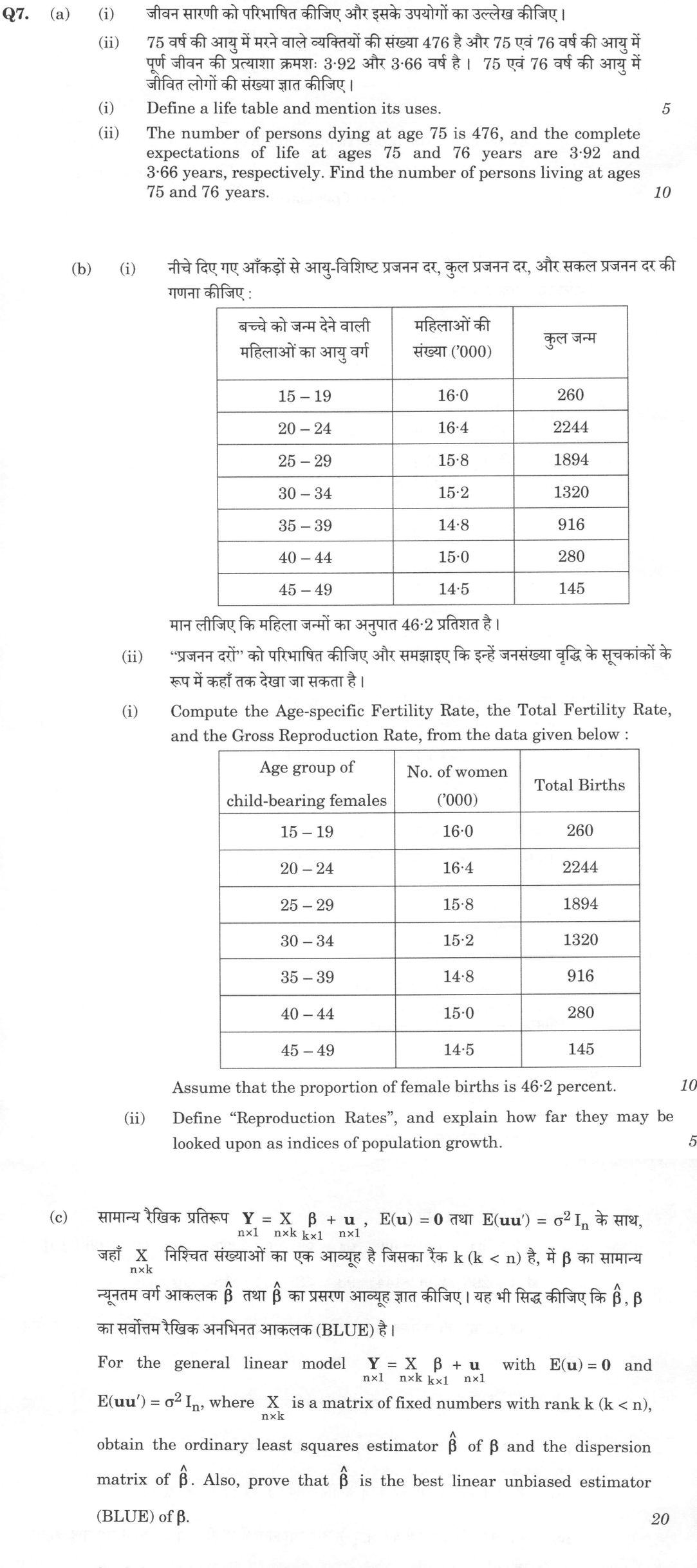
(a) (i) Define a life table and mention its uses. (5 marks) (ii) The number of persons dying at age 75 is 476, and the complete…

(a)(i) Life table and its uses (5 marks)

A life table is a statistical table showing how a hypothetical cohort (radix l₀, usually 100,000 births) diminishes with age under a fixed set of age-specific mortality rates, and so summarises the mortality experience of a population. Its columns are lₓ (survivors at age x), dₓ = lₓ − lₓ₊₁ (deaths), qₓ = dₓ/lₓ and pₓ = 1 − qₓ (probabilities of dying and surviving), Lₓ (person-years lived between x and x + 1), Tₓ (person-years lived above x) and eₓ = Tₓ/lₓ (expectation of life). Assumptions: a closed cohort with no migration, mortality rates constant in time, and deaths spread uniformly within each year of age. Uses: computing life expectancy and comparing mortality across regions and periods; premiums and annuities in insurance and pension planning; population projections and survival ratios; building stable-population models and net reproduction rates; and planning health services.

(a)(ii) Persons living at ages 75 and 76 (10 marks)

With deaths spread uniformly in a year, the complete expectation of life satisfies eₓ = ½ + pₓ(eₓ₊₁ + ½) (the curtate expectation is pₓ(1 + e^cₓ₊₁), and eₓ = eₓ^c + ½).

Hence p₇₅ = (e₇₅ − ½)/(e₇₆ + ½) = (3.92 − 0.5)/(3.66 + 0.5) = 3.42/4.16 = 0.8221, and q₇₅ = 1 − p₇₅ = 0.1779.

Since d₇₅ = l₇₅ q₇₅ = 476, l₇₅ = 476/0.1779 = 2,676 (approximately, 2,675.9).

Then l₇₆ = l₇₅ − d₇₅ = 2,676 − 476 = 2,200 (check: 2,676 × 0.8221 = 2,200).

So the number living at age 75 is about 2,676 and at age 76 about 2,200.

(b)(i) Fertility rates (10 marks)

Age-specific fertility rate, ASFR = births to women of the group/number of women in the group × 1,000. The women are in thousands, so for 15-19: 260/16,000 × 1,000 = 16.25.

Age group, ASFR per 1,000:

• 15-19: 260/16,000 = 16.25
• 20-24: 2,244/16,400 = 136.83
• 25-29: 1,894/15,800 = 119.87
• 30-34: 1,320/15,200 = 86.84
• 35-39: 916/14,800 = 61.89
• 40-44: 280/15,000 = 18.67
• 45-49: 145/14,500 = 10.00

The sum of ASFRs is 450.35 per 1,000. Total fertility rate TFR = 5 × ΣASFR (five-year groups) = 5 × 450.35/1,000 = 2.252 births per woman (or 2,252 per 1,000 women).

Gross reproduction rate GRR = TFR × proportion of female births = 2.252 × 0.462 = 1.040 daughters per woman. (Equivalently, ASFRs of female births are 7.51, 63.22, 55.38, 40.12, 28.59, 8.62, 4.62, which sum to 208.06 and give 5 × 0.20806 = 1.040.)

(b)(ii) Reproduction rates as indices of population growth (5 marks)

The gross reproduction rate is the average number of daughters a woman would bear in her lifetime if she experienced the current age-specific fertility rates and all survived to the end of the reproductive period. The net reproduction rate (NRR) allows for mortality: NRR = Σ fₓ (Lₓ/l₀), the number of daughters who would survive to their mother's age at birth.

As indices of growth: NRR = 1 means exact replacement and eventual zero growth, NRR > 1 growth and NRR < 1 decline; the long-run growth rate is r ≈ ln(NRR)/T, with T the mean generation length. They are better than crude rates because they are not affected by age structure. But they are limited: they describe eventual, not current, growth, since a young age structure carries momentum for decades; they assume constant fertility and mortality; they ignore migration and males; and tempo effects can distort period measures. Thus they are indices of replacement rather than exact indicators of population growth. GRR overstates because it ignores mortality.

(c) OLS estimator, dispersion matrix and BLUE property (20 marks)

Model: Y = Xβ + u, E(u) = 0, E(uu′) = σ²Iₙ, X fixed with rank k, so X′X is non-singular.

Estimator: minimise S = (Y − Xβ)′(Y − Xβ) = Y′Y − 2β′X′Y + β′X′Xβ. Setting ∂S/∂β = −2X′Y + 2X′Xβ = 0 gives the normal equations X′Xβ̂ = X′Y, so β̂ = (X′X)⁻¹X′Y. The second derivative 2X′X is positive definite, so this is a minimum.

Unbiasedness: β̂ = (X′X)⁻¹X′(Xβ + u) = β + (X′X)⁻¹X′u, so E(β̂) = β.

Dispersion matrix: β̂ − β = (X′X)⁻¹X′u, so D(β̂) = E[(X′X)⁻¹X′uu′X(X′X)⁻¹] = (X′X)⁻¹X′(σ²Iₙ)X(X′X)⁻¹ = σ²(X′X)⁻¹.

BLUE (Gauss-Markov): let β* = CY be any linear estimator, and write C = (X′X)⁻¹X′ + D, D an arbitrary k × n matrix. E(β*) = CXβ = β + DXβ, which equals β for all β only if DX = 0. Under this condition, β* − β = Cu = [(X′X)⁻¹X′ + D]u, and

D(β*) = σ²CC′ = σ²[(X′X)⁻¹X′X(X′X)⁻¹ + (X′X)⁻¹X′D′ + DX(X′X)⁻¹ + DD′] = σ²[(X′X)⁻¹ + DD′],

since the cross terms vanish because DX = 0 (and X′D′ = 0). Therefore D(β*) − D(β̂) = σ²DD′, which is positive semi-definite, so for every vector λ, Var(λ′β*) ≥ Var(λ′β̂), with equality only when D = 0. Thus β̂ has the minimum variance among linear unbiased estimators of every linear function of β; it is BLUE.