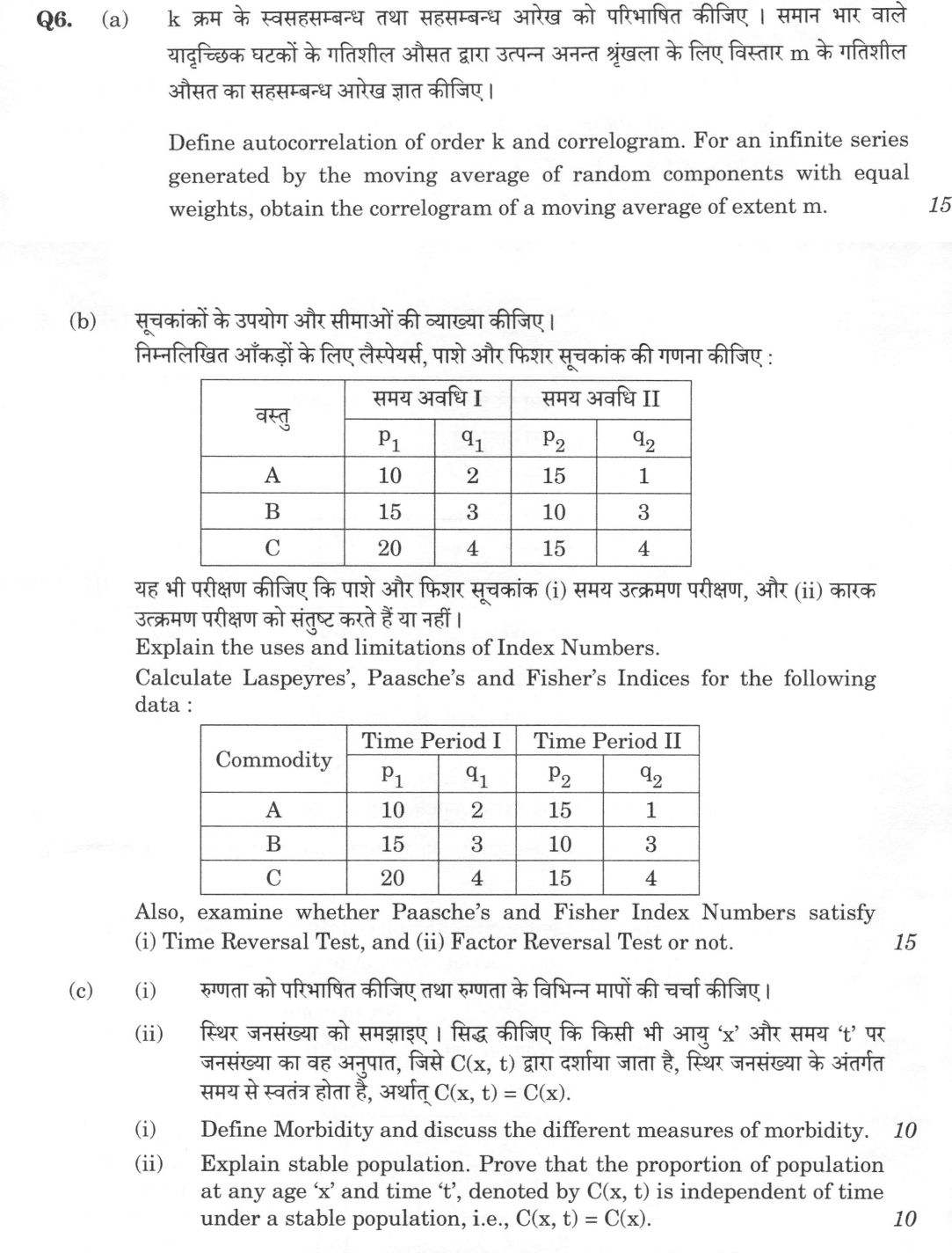
(a) Define autocorrelation of order k and correlogram. For an infinite series generated by the moving average of random…

(a) Autocorrelation, correlogram and the moving-average series (15 marks)

The autocorrelation of order k of a stationary series is ρₖ = γₖ/γ₀ = Cov(xₜ, xₜ₊ₖ)/Var(xₜ), the correlation between observations k periods apart, with ρ₀ = 1 and ρ₋ₖ = ρₖ. The correlogram is the plot of ρₖ (sample estimates rₖ) against the lag k = 0, 1, 2, …; it displays the structure of the series and is used to identify its type, for example a slowly damped pattern for a trend, oscillation for a seasonal or cyclical series, and rapid fall to zero for a random series.

Let εₜ be uncorrelated random components with mean 0 and variance σ², and let the series be the equal-weight moving average of extent m:

xₜ = (1/m)(εₜ + εₜ₋₁ + … + εₜ₋ₘ₊₁).

Then E(xₜ) = 0 and γ₀ = Var(xₜ) = m σ²/m² = σ²/m. For lag k, xₜ and xₜ₊ₖ have the terms εₜ₊ₖ, …, εₜ₊ₖ₋ₘ₊₁ and εₜ, …, εₜ₋ₘ₊₁, which share the m − k random components common to both windows when k < m, and none when k ≥ m. Hence

γₖ = (m − k)σ²/m² for k ≤ m, and γₖ = 0 for k ≥ m,

and therefore

ρₖ = γₖ/γ₀ = (m − k)/m = 1 − k/m for 0 ≤ k ≤ m; ρₖ = 0 for k ≥ m.

The correlogram is thus a straight line falling from 1 at k = 0 to 0 at k = m (a triangle), and zero beyond the lag m. The figure shows the case m = 6, where ρₖ = 1, 5/6, 4/6, 3/6, 2/6, 1/6, 0. The oscillations and correlations that a moving average creates in a purely random series are the Slutsky-Yule effect: the series is autocorrelated although its underlying components are independent.

(b) Index numbers: uses, limitations and calculation (15 marks)

Uses: index numbers measure relative changes in prices, quantities or values over time or place; they act as economic barometers (the CPI, WPI and IIP), are used for deflating nominal values to real values, for indexing wages and dearness allowance, for policy and forecasting, and for comparing standards of living.

Limitations: they are only approximate averages; the choice of base year, of items and of weights affects the result, and old weights become out of date; different formulae give different answers, with substitution bias in the Laspeyres index; quality changes and new goods are hard to capture; and an index for one group or place may not be valid for another.

Calculation, with base period I and current period II. Σp₁q₁ = 10·2 + 15·3 + 20·4 = 145; Σp₂q₁ = 15·2 + 10·3 + 15·4 = 120; Σp₁q₂ = 10·1 + 15·3 + 20·4 = 135; Σp₂q₂ = 15·1 + 10·3 + 15·4 = 105.

Laspeyres P_L = Σp₂q₁/Σp₁q₁ × 100 = 120/145 × 100 = 82.76. Paasche P_P = Σp₂q₂/Σp₁q₂ × 100 = 105/135 × 100 = 77.78. Fisher P_F = √(P_L × P_P) = √(0.8276 × 0.7778) × 100 = 80.23.

Time reversal test: P₀₁ × P₁₀ = 1. For Fisher, P₁₀ = √[(Σp₁q₂/Σp₂q₂)(Σp₁q₁/Σp₂q₁)] = 1/P₀₁, so the test is satisfied. For Paasche, P₀₁ = 105/135 = 0.7778 and P₁₀ = Σp₁q₁/Σp₂q₁ = 145/120 = 1.2083, and the product is 0.9398 ≠ 1, so the test fails.

Factor reversal test: P₀₁ × Q₀₁ = Σp₂q₂/Σp₁q₁ = 105/145 = 0.7241. For Fisher, Q₀₁ = √[(Σp₁q₂/Σp₁q₁)(Σp₂q₂/Σp₂q₁)] = √(0.9310 × 0.8750) = 0.9026, and 0.8023 × 0.9026 = 0.7241, so it is satisfied. For Paasche, Q₀₁ = Σp₂q₂/Σp₂q₁ = 105/120 = 0.875, and 0.7778 × 0.875 = 0.6806 ≠ 0.7241, so it fails. Hence Fisher's index satisfies both tests, whereas Paasche satisfies neither.

(c)(i) Morbidity and its measures (10 marks)

Morbidity is any departure, subjective or objective, from a state of physiological or psychological well-being, so that illness, injury or disability is present. It is measured by:

• Incidence rate: new cases occurring in a period divided by the population at risk, times a constant (for example 1,000). It measures the risk of falling ill.
• Prevalence: all existing cases (old and new) divided by population, at a point in time (point prevalence) or over a period (period prevalence). Approximately prevalence = incidence × average duration.
• Attack rate: cases among those exposed during an epidemic, and secondary attack rate among contacts.
• Case-fatality rate: deaths from a disease divided by the cases of that disease; and the duration of illness.
• Disability-based measures: days of disability or sickness absence, disability-free life expectancy, and the composite DALY (years of life lost plus years lived with disability) and its Sullivan-method relatives.
• Sources are surveys (NSS, NFHS, self-reports), hospital records and disease registries, with limitations from reporting bias and differing definitions.

(c)(ii) Stable population and C(x, t) = C(x) (10 marks)

A stable population is one that has had constant age-specific fertility and mortality rates for a long time and is closed to migration; it grows or declines at a constant rate r, and its age distribution is fixed. Let l(a) be the survival function from birth (l(0) = 1) and B(t) the annual births. By Lotka's renewal equation B(t) = ∫B(t − a)l(a)m(a)da, with m(a) the maternity function fixed; its solution is B(t) = B(0)e^rt, where r is the real root of ∫e^-ral(a)m(a)da = 1.

Persons aged x at time t are those born at t − x who have survived to x, so N(x, t) = B(t − x)l(x) = B(0)e^r(t − x)l(x). The total population is N(t) = ∫₀^ω N(a, t)da = B(0)e^rt∫₀^ω e^-ral(a)da. Hence the proportion at age x is

C(x, t) = N(x, t)/N(t) = e^-rxl(x)/∫₀^ω e^-ral(a)da,

in which t does not appear. Thus C(x, t) = C(x), independent of time: the age distribution of a stable population is constant, and it depends only on r and the survival function.