Paper II — Q3
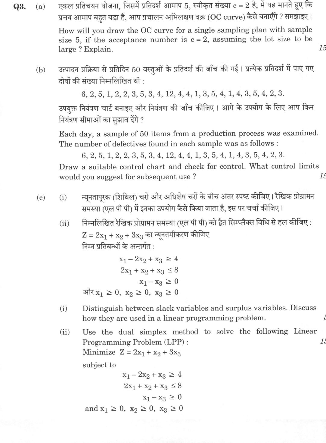
(a) How will you draw the OC curve for a single sampling plan with sample size 5, if the acceptance number is c = 2, assuming the…
How will you draw the OC curve for a single sampling plan with sample size 5, if the acceptance number is c = 2, assuming the lot size to be large ? Explain. 15 marks
Each day, a sample of 50 items from a production process was examined. The number of defectives found in each sample was as follows : 6, 2, 5, 1, 2, 2, 3, 5, 3, 4, 12, 4, 4, 1, 3, 5, 4, 1, 4, 3, 5, 4, 2, 3. Draw a suitable control chart and check for control. What control limits would you suggest for subsequent use ? 15 marks
Distinguish between slack variables and surplus variables. Discuss how they are used in a linear programming problem. 5 marks
Use the dual simplex method to solve the following Linear Programming Problem (LPP) : Minimize Z = 2x₁ + x₂ + 3x₃ subject to x₁ − 2x₂ + x₃ ≥ 4 2x₁ + x₂ + x₃ ≤ 8 x₁ − x₃ ≥ 0 and x₁ ≥ 0, x₂ ≥ 0, x₃ ≥ 0 15 marks
हिंदी में प्रश्न पढ़ें
एकल प्रतिचयन योजना, जिसमें प्रतिदर्श आमाप 5, स्वीकृत संख्या c = 2 है, में यह मानते हुए कि प्रचय आमाप बहुत बड़ा है, आप प्रचालन अभिलक्षण वक्र (OC curve) कैसे बनाएँगे ? समझाइए । (15 अंक)
उत्पादन प्रक्रिया से प्रतिदिन 50 वस्तुओं के प्रतिदर्श की जाँच की गई । प्रत्येक प्रतिदर्श में पाए गए दोषों की संख्या निम्नलिखित थी : 6, 2, 5, 1, 2, 2, 3, 5, 3, 4, 12, 4, 4, 1, 3, 5, 4, 1, 4, 3, 5, 4, 2, 3. उपयुक्त नियंत्रण चार्ट बनाइए और नियंत्रण की जाँच कीजिए । आगे के उपयोग के लिए आप किन नियंत्रण सीमाओं का सुझाव देंगे ? (15 अंक)
न्यूनतापूरक (शिथिल) चरों और अधिशेष चरों के बीच अंतर स्पष्ट कीजिए । रैखिक प्रोग्रामन समस्या (एल पी पी) में इनका उपयोग कैसे किया जाता है, इस पर चर्चा कीजिए । (5 अंक)
निम्नलिखित रैखिक प्रोग्रामन समस्या (एल पी पी) को द्वैत सिम्प्लेक्स विधि से हल कीजिए : Z = 2x₁ + x₂ + 3x₃ का न्यूनतमीकरण कीजिए निम्न प्रतिबन्धों के अन्तर्गत : x₁ − 2x₂ + x₃ ≥ 4 2x₁ + x₂ + x₃ ≤ 8 x₁ − x₃ ≥ 0 और x₁ ≥ 0, x₂ ≥ 0, x₃ ≥ 0 (15 अंक)
Model answer
Drafted with AI by UPSC Answer Check against this question's marking rubric, to the expected length. UPSC does not publish answers for Mains — this is one way to score well, not an official key. How we build rubrics and answers.
(a) OC curve for the plan n = 5, c = 2
For a single sampling plan with sample size n = 5 and acceptance number c = 2, the Operating Characteristic (OC) curve is drawn from the probability of accepting a lot of incoming quality p. Because the lot size N is assumed very large, the draws are effectively independent and with replacement, so the Type‑B binomial model (not the hypergeometric) is the correct sampling distribution. A lot is accepted when the number of defectives d in the sample does not exceed c, so the acceptance probability is the cumulative binomial probability P(d ≤ 2):
Pₐ(p) = Σ_d=0² C(5, d) pᵈ (1 − p)⁵⁻ᵈ = (1−p)⁵ + 5p(1−p)⁴ + 10p²(1−p)³.
To plot the curve, Pₐ is evaluated over a spread of p values and the points (p, Pₐ) are joined:
| p | 0.05 | 0.10 | 0.20 | 0.30 | 0.50 |
|---|---|---|---|---|---|
| Pₐ | 0.9988 | 0.9914 | 0.9421 | 0.8369 | 0.5000 |
Plotting Pₐ on the vertical axis against the lot fraction defective p on the horizontal axis gives a smooth, downward‑sloping curve. It encodes the two risks: at the Acceptable Quality Level (AQL) the curve equals 1 − α (α = producer's risk), and at the Lot Tolerance Percent Defective (LTPD) it equals β (consumer's risk). The ideal OC curve is a vertical step at p = c/n = 0.4; here, with n = 5 the curve is very flat (Pₐ is still 0.94 at p = 0.20), so the plan has poor discriminating power. Increasing n steepens the curve toward the ideal step, whereas increasing c merely shifts the curve upward (easier acceptance).

(b) np chart for the number of defectives
The data record the number of defectives out of a fixed daily sample of n = 50, a binomial situation, so the suitable chart is the np chart (equivalently a p chart). Over the 24 samples the total number of defectives is 88, so p̄ = 88/1200 = 0.0733 and the centre line is n p̄ = 3.667. The binomial standard deviation is σₙₚ = √(n p̄ (1 − p̄)) = √(3.667 × 0.9267) = 1.843, giving trial 3‑sigma limits UCL = 3.667 + 3(1.843) = 9.20 and LCL = 3.667 − 3(1.843) = −1.86, which is replaced by 0. Plotting the 24 points against these limits, sample 11 (12 defectives) lies above the UCL of 9.20; a single point outside the limits means the process is out of statistical control, so an assignable cause must be investigated and that point removed. For subsequent use the limits are recomputed from the remaining 23 samples: new total = 88 − 12 = 76, so n p̄ = 76/23 = 3.304 (p̄ = 0.0661) and σₙₚ = √(3.304 × 0.9339) = 1.755. The revised limits are UCL = 3.304 + 3(1.755) = 8.57 and LCL = 3.304 − 3(1.755) = −1.96 → 0 (on the p‑chart scale, p̄ = 0.0661, UCL = 0.1715). These tightened limits are recommended for ongoing monitoring once the assignable cause is eliminated.

(c) (i) Slack versus surplus variables
Slack and surplus variables are non‑negative variables added to the objective with zero coefficient to turn inequalities into equalities. A slack variable is added to a "≤" constraint (unused resource); a surplus variable is subtracted from a "≥" constraint (over‑fulfilment of a requirement). A slack column forms part of the identity matrix, giving a ready initial basic feasible solution, whereas a surplus column has coefficient −1 and cannot start the basis, so an artificial variable must be introduced (Big‑M or Two‑Phase method). At the optimum, complementary slackness links a positive slack/surplus to a non‑binding constraint with zero shadow price.
(c) (ii) Dual simplex solution
The dual simplex method requires a dual‑feasible (cⱼ − zⱼ ≥ 0) but primal‑infeasible (negative RHS) start. Multiply the "≥" constraints (1) and (3) by −1 so all rows are "≤": −x₁ + 2x₂ − x₃ ≤ −4; 2x₁ + x₂ + x₃ ≤ 8; −x₁ + x₃ ≤ 0. Adding slacks s₁, s₂, s₃ (no artificial variables are needed) gives the initial tableau, basis (s₁, s₂, s₃), with cⱼ − zⱼ = (2, 1, 3, 0, 0, 0) ≥ 0 and RHS (−4, 8, 0):
| Basis | x₁ | x₂ | x₃ | s₁ | s₂ | s₃ | RHS |
|---|---|---|---|---|---|---|---|
| s₁ | −1 | 2 | −1 | 1 | 0 | 0 | −4 |
| s₂ | 2 | 1 | 1 | 0 | 1 | 0 | 8 |
| s₃ | −1 | 0 | 1 | 0 | 0 | 1 | 0 |
| cⱼ − zⱼ | 2 | 1 | 3 | 0 | 0 | 0 | Z = 0 |
Iteration 1. Leaving variable = most negative basic value, s₁ = −4 (row 1). Entering variable = min (cⱼ − zⱼ)/|a₁ⱼ| over negative a₁ⱼ only: x₁ → 2/1 = 2, x₃ → 3/1 = 3; minimum 2, so x₁ enters. Pivot on −1. After row operations the tableau becomes, basis (x₁, s₂, s₃):
| Basis | x₁ | x₂ | x₃ | s₁ | s₂ | s₃ | RHS |
|---|---|---|---|---|---|---|---|
| x₁ | 1 | −2 | 1 | −1 | 0 | 0 | 4 |
| s₂ | 0 | 5 | −1 | 2 | 1 | 0 | 0 |
| s₃ | 0 | −2 | 2 | −1 | 0 | 1 | 4 |
| cⱼ − zⱼ | 0 | 5 | 1 | 2 | 0 | 0 | Z = 8 |
All right‑hand sides are now non‑negative (primal feasible) and all cⱼ − zⱼ remain non‑negative (dual feasible), so the solution is optimal in a single iteration. Reading off the basics: x₁ = 4, s₂ = 0, s₃ = 4, with non‑basics x₂ = x₃ = s₁ = 0. Hence x₁ = 4, x₂ = 0, x₃ = 0 and Z_min = 8. Verification in the original constraints: 4 − 0 + 0 = 4 ≥ 4; 8 + 0 + 0 = 8 ≤ 8; 4 − 0 = 4 ≥ 0 — all satisfied, confirming the optimum.
How this answer will be evaluated
Evaluation rubric
Each sub-part is marked on its own, against the marks and word limit printed on the paper.
- (a) Explain how the operating characteristic (OC) curve of a single sampling plan with n = 5 and c = 2 is constructed when the lot size is large. The answer must state the sampling distribution to use (binomial, since N is large), give the acceptance-probability function, tabulate P_a for a range of incoming quality levels p, describe the plot, and interpret the curve (AQL, LTPD, producer's and consumer's risks, effect of n and c). 15 marks
Must cover
- Type-B OC curve; binomial model justified by large lot size
- P_a(p) = (1-p)^5 + 5p(1-p)^4 + 10p^2(1-p)^3
- Table of P_a: 0.9988 at p = 0.05; 0.9914 at 0.10; 0.9421 at 0.20; 0.8369 at 0.30; 0.5000 at 0.50
- AQL, LTPD, producer's risk alpha, consumer's risk beta
- Ideal OC curve is a vertical step; finite n makes the curve flat
Loses marks
- Using the hypergeometric distribution: with a large lot the type-B binomial curve is correct and is what the question's 'assuming the lot size to be large' signals
- Computing P(d = 2) instead of the cumulative P(d <= 2) - the acceptance number c = 2 means 0, 1 or 2 defectives are acceptable
- Plotting P_a against d, or against n, instead of against the lot fraction defective p
- Tabulating only two or three points, which cannot define a curve; at least five well-spread p values are needed
- Claiming that increasing c makes the curve steeper - increasing c shifts the curve UP (makes acceptance easier); only increasing n steepens it
Earns more
- Interprets the curve in terms of AQL (P_a = 1 - alpha), LTPD (P_a = beta), producer's risk alpha and consumer's risk beta
- Comments on discriminating power: the n = 5 curve is very flat (P_a = 0.94 even at p = 0.20); increasing n steepens the curve towards the ideal step at p = c/n, while increasing c raises it
- (b) Three demands: (i) choose and construct the suitable control chart for 24 daily samples of constant size n = 50 with the number of defectives recorded - this is an np chart (equivalently a p chart); (ii) test whether the process is in statistical control; (iii) recommend revised control limits for subsequent use after eliminating any assignable cause. 15 marks
Must cover
- np chart (or p chart) with constant n = 50
- Sum of defectives = 88, p-bar = 0.0733, n p-bar = 3.667
- Trial UCL = 9.20, LCL = 0
- Sample 11 (12 defectives) is out of control
- Revised n p-bar = 3.304, UCL = 8.57, LCL = 0 (p-chart: p-bar = 0.0661, UCL = 0.1715)
- 3-sigma limits based on the binomial standard deviation
Loses marks
- Using a c chart or u chart: the data are the number of DEFECTIVE ITEMS out of a fixed 50 inspected, which is binomial (np chart), not the number of defects per unit (Poisson)
- Arithmetic error in summing the 24 values - the correct total is 88; a wrong total corrupts every subsequent figure
- Reporting a negative LCL (-1.86) instead of setting it to zero
- Declaring the process in control because 'most points are inside' - a single point outside the limits means out of control
- Failing to answer the third demand (revised limits for subsequent use), which carries a full 3 marks, or revising without first removing the out-of-control point
Earns more
- Computes sum of defectives = 88 over 24 samples, p-bar = 88/1200 = 0.0733 and n p-bar = 3.667
- Computes trial limits UCL = 3.667 + 3(1.8433) = 9.197 and LCL = -1.863 set to 0, and notes that a negative LCL is replaced by zero
- (c)(i) Distinguish slack from surplus variables and discuss the role each plays in formulating and solving a linear programming problem (conversion to standard form, starting basis, need for artificial variables, economic interpretation). 5 marks
Must cover
- Slack added to 'less than or equal to'; surplus subtracted from 'greater than or equal to'
- Both >= 0, zero coefficient in the objective function
- Slack columns form the identity matrix / initial basic feasible solution
- Artificial variable, Big-M (penalty) method, Two-Phase method
- Complementary slackness / shadow price interpretation
Loses marks
- Reversing the two: adding a variable to a 'greater than or equal to' constraint or subtracting from a 'less than or equal to'
- Confusing a surplus variable with an artificial variable - the surplus is a genuine decision-relevant variable, the artificial is a computational device removed in Phase I
- Giving slack/surplus a non-zero objective coefficient
- Answering only the definitional part and omitting the 'how they are used' discussion, which is half the question
- Saying that surplus variables can be negative because they are subtracted - all variables in standard form are non-negative
Earns more
- Both are non-negative and enter the objective function with coefficient zero
- Economic/duality interpretation: positive slack at the optimum means a non-binding constraint with zero shadow price (complementary slackness); positive surplus means over-fulfilment of a requirement
- (c)(ii) Solve the given minimisation LPP by the DUAL SIMPLEX method specifically - convert all constraints to the 'less than or equal to' form, set up a dual-feasible but primal-infeasible starting tableau, and iterate using the dual-simplex leaving-then-entering rule until primal feasibility is attained. State the optimal x1, x2, x3 and Z. 15 marks
Must cover
- Dual simplex: start dual feasible (c_j - z_j >= 0) and primal infeasible (negative RHS)
- Multiply 'greater than or equal to' rows by -1; slacks s1, s2, s3; no artificial variables needed
- Leaving variable = most negative basic value (s1 = -4)
- Entering variable = min |(c_j - z_j)/a_rj| over negative a_rj only; x1 enters with ratio 2
- Optimal x1 = 4, x2 = 0, x3 = 0
- Z_min = 8
Loses marks
- Forgetting to multiply the 'greater than or equal to' rows by -1, so the starting basis is not primal infeasible and the dual simplex cannot be started
- Using the ORDINARY simplex ratio test (RHS / column entry over positive entries) instead of the dual ratio |(c_j - z_j)/a_rj| over NEGATIVE row entries
- Including positive or zero entries of the pivot row in the dual ratio test - only strictly negative a_rj are eligible
- Introducing artificial variables and the Big-M method, which answers a different question - the paper demands the dual simplex method
- Stopping at x1 = 4 without checking that all c_j - z_j remain non-negative, or without verifying the solution in the ORIGINAL constraints
Earns more
- Applies the dual-simplex leaving rule correctly: the row with the most negative basic value (s1 = -4) leaves
- Performs the pivot correctly, obtaining the tableau x1 = 4, s2 = 0, s3 = 4 with all right-hand sides non-negative and all c_j - z_j still non-negative, hence optimal
What "Explain" is asking you to do
Make the working of something clear — what sets it off, what follows from what, and what it produces. Explain is the Commission's mechanism word: it dominates the technical papers and the “explain why” stems, where the marks sit in the causal chain and not in the label.
Structure that answers it
State what it is → the initiating condition → the chain of cause, step by step → an instance where it plays out → what the chain produces
Where marks are lost
Describing what something looks like instead of why it works that way. Naming the stages without linking them reads as description too.
Practice this exact question
Write your answer and it is marked point by point against the model answer above — what you covered, what you missed, what you got wrong.
Evaluate my answer →More from Statistics 2026 Paper II
- Q1 (a) Suppose that a given individual in a population has a survival time which is exponent…
- Q2 (a) (i) Describe the construction of a CUSUM chart with Decision interval and Reference v…
- Q3 (a) How will you draw the OC curve for a single sampling plan with sample size 5, if the…
- Q4 (a) (i) Discuss the theoretical basis of the sequential probability ratio test (SPRT) in…
- Q5 (a) Explain the 2-stage least squares (2SLS) method of estimation for the following simul…
- Q6 (a) Define autocorrelation of order k and correlogram. For an infinite series generated b…