Paper I — Q8
(a) (i) The melting point of tin is 232°C, its latent heat of fusion is 14 cal/g and the specific heat of solid and molten tin…
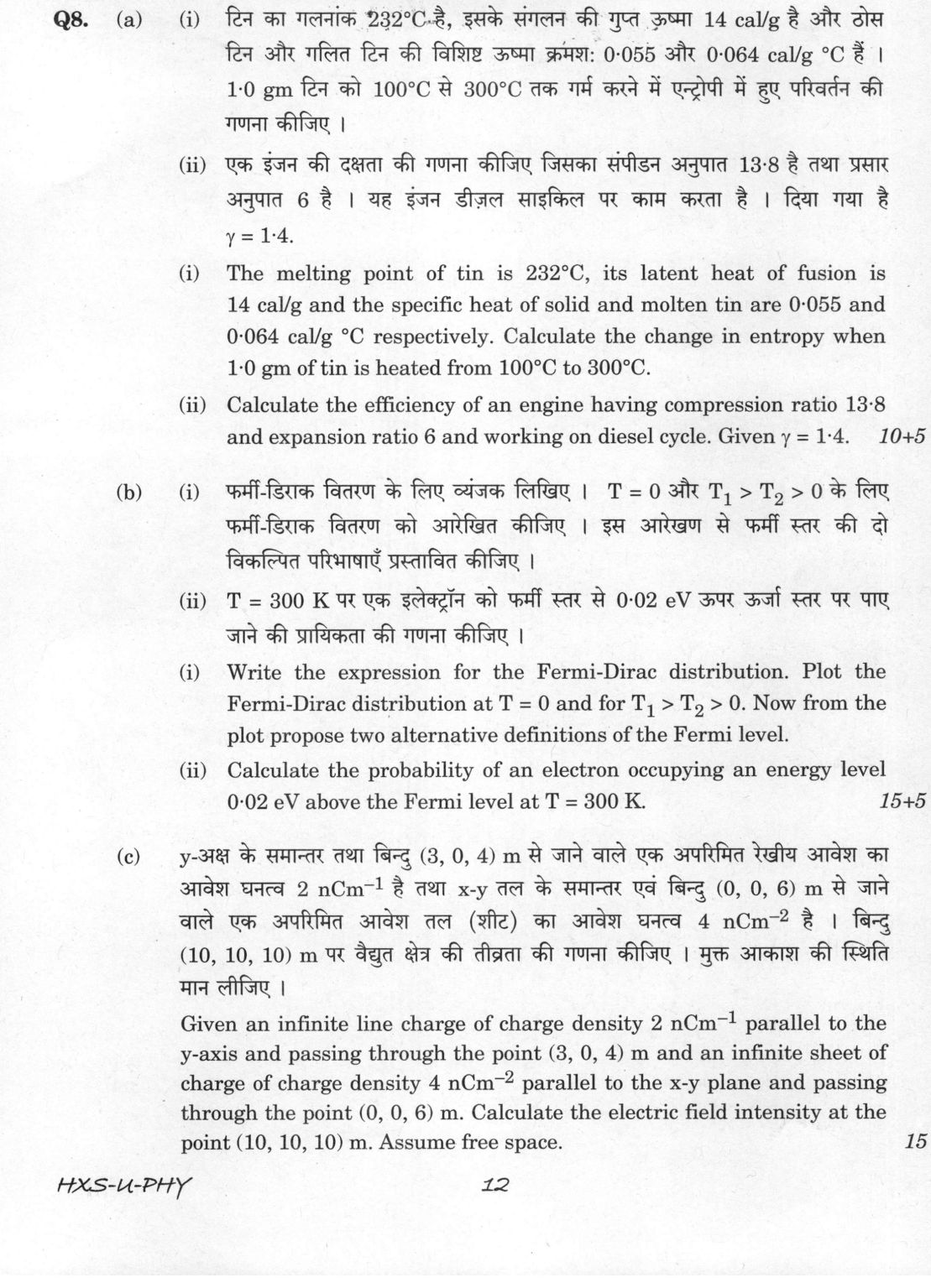
The melting point of tin is 232°C, its latent heat of fusion is 14 cal/g and the specific heat of solid and molten tin are 0·055 and 0·064 cal/g °C respectively. Calculate the change in entropy when 1·0 gm of tin is heated from 100°C to 300°C.
Calculate the efficiency of an engine having compression ratio 13·8 and expansion ratio 6 and working on diesel cycle. Given γ = 1·4. (10+5 marks)
Write the expression for the Fermi-Dirac distribution. Plot the Fermi-Dirac distribution at T = 0 and for T₁ > T₂ > 0. Now from the plot propose two alternative definitions of the Fermi level.
Calculate the probability of an electron occupying an energy level 0·02 eV above the Fermi level at T = 300 K. (15+5 marks)
Given an infinite line charge of charge density 2 nCm⁻¹ parallel to the y-axis and passing through the point (3, 0, 4) m and an infinite sheet of charge of charge density 4 nCm⁻² parallel to the x-y plane and passing through the point (0, 0, 6) m. Calculate the electric field intensity at the point (10, 10, 10) m. Assume free space. 15 marks
हिंदी में प्रश्न पढ़ें
टिन का गलनांक 232°C है, इसके संगलन की गुप्त ऊष्मा 14 cal/g है और ठोस टिन और गलित टिन की विशिष्ट ऊष्मा क्रमशः 0·055 और 0·064 cal/g °C हैं । 1·0 gm टिन को 100°C से 300°C तक गर्म करने में एन्ट्रॉपी में हुए परिवर्तन की गणना कीजिए ।
एक इंजन की दक्षता की गणना कीजिए जिसका संपीडन अनुपात 13·8 है तथा प्रसार अनुपात 6 है । यह इंजन डीजल साइकिल पर काम करता है । दिया गया है γ = 1·4. (10+5 अंक)
फर्मी-डिराक वितरण के लिए व्यंजक लिखिए । T = 0 और T₁ > T₂ > 0 के लिए फर्मी-डिराक वितरण को आरेखित कीजिए । इस आरेखण से फर्मी स्तर की दो विकल्पित परिभाषाएँ प्रस्तावित कीजिए ।
T = 300 K पर एक इलेक्ट्रॉन को फर्मी स्तर से 0·02 eV ऊपर ऊर्जा स्तर पर पाए जाने की प्रायिकता की गणना कीजिए । (15+5 अंक)
y-अक्ष के समांतर तथा बिंदु (3, 0, 4) m से जाने वाले एक अपरिमित रेखीय आवेश का आवेश घनत्व 2 nCm⁻¹ है तथा x-y तल के समांतर एवं बिंदु (0, 0, 6) m से जाने वाले एक अपरिमित आवेश तल (शीट) का आवेश घनत्व 4 nCm⁻² है । बिंदु (10, 10, 10) m पर वैद्युत क्षेत्र की तीव्रता की गणना कीजिए । मुक्त आकाश की स्थिति मान लीजिए । (15 अंक)
Model answer
Written by UPSC Answer Check against this question's marking rubric, to the expected length. UPSC does not publish answers for Mains — this is one way to score well, not an official key.
(a)(i) Entropy is a state function, so evaluate ΔS along a reversible path: heat solid to melting point, melt it, heat liquid to 300°C. T₁ = 100 + 273.15 = 373.15 K, T_m = 232 + 273.15 = 505.15 K, T₂ = 300 + 273.15 = 573.15 K. For m = 1.0 g:
- ΔS₁ = ∫_T₁^T_m m c_s dT/T = m c_s ln(T_m/T₁) = 1.0 × 0.055 × ln(505.15/373.15) = 0.01666 cal/K.
- ΔS₂ = m L/T_m = 1.0 × 14/505.15 = 0.02771 cal/K.
- ΔS₃ = ∫_T_m^T₂ m c_l dT/T = m c_l ln(T₂/T_m) = 1.0 × 0.064 × ln(573.15/505.15) = 0.00808 cal/K.
Total entropy change: ΔS = 0.01666 + 0.02771 + 0.00808 = 0.05245 cal/K = 0.05245 × 4.184 = 0.2195 J/K.
Condition: pressure constant and phase changes reversible. Final answer: ΔS ≈ 0.0525 cal/K = 0.220 J/K.
(a)(ii) For an ideal air-standard Diesel cycle, let compression ratio r = V₁/V₂ = 13.8 and expansion ratio R = V₄/V₃ = 6. Then cut-off ratio ρ = V₃/V₂ = r/R = 13.8/6 = 2.3. Efficiency: η = 1 − [1/(γ r^(γ−1))] × [(ρ^γ − 1)/(ρ − 1)].
Given γ = 1.4: r^(γ−1) = 13.8^0.4 = 2.8573, ρ^γ = 2.3^1.4 = 3.2094.
Thus: η = 1 − [(3.2094 − 1)/(1.4 × 2.8573 × (2.3 − 1))] = 1 − [2.2094/(1.4 × 2.8573 × 1.3)] = 1 − 0.42486 = 0.57514.
So η ≈ 57.5%.
(b)(i) The Fermi-Dirac distribution is: f(E) = 1/[exp((E − E_F)/(k_B T)) + 1], where f(E) is the probability that a state of energy E is occupied.
Plot description: take E on the horizontal axis and f(E) on the vertical axis. At T = 0, the curve is a step: f(E) = 1 for E < E_F, f(E) = 0 for E > E_F, and conventionally f(E_F) = 1/2. For T > 0, the step becomes smooth. At E = E_F, f(E_F) = 1/2 for every finite T > 0. For T₁ > T₂ > 0, the curve for T₁ is more spread out; it lies above the T₂ curve for E > E_F and below it for E < E_F. The rounding width is of order k_B T.
Two alternative definitions of the Fermi level from the plot:
- The energy at which the occupation probability is exactly 1/2 at any finite temperature T > 0.
- The limiting energy at T → 0 at which the occupation drops from 1 to 0, i.e. the energy separating occupied and unoccupied states.
(b)(ii) Given ΔE = E − E_F = 0.02 eV, T = 300 K. k_B T = 8.617 × 10⁻⁵ × 300 = 0.02585 eV.
Then: f = 1/[exp(ΔE/k_B T) + 1] = 1/[exp(0.02/0.02585) + 1] = 1/[exp(0.7736) + 1] = 1/(2.1676 + 1) = 0.3157.
So the probability is f ≈ 0.316 = 31.6%.
(c) Use superposition of the fields due to the infinite line charge and the infinite sheet charge.
For the line charge: λ = 2 nC/m = 2 × 10⁻⁹ C/m. It is parallel to the y-axis and passes through (3, 0, 4) m. At P = (10, 10, 10) m, the perpendicular displacement from the line in the x-z plane is: r = (10 − 3)î + (10 − 4)k̂ = 7î + 6k̂. Distance d = √(7² + 6²) = √85 m.
By Gauss’s law for an infinite line charge: E_line = λ/(2π ε₀ d) r̂ = λ/(2π ε₀ d²) r = [2 × 10⁻⁹/(2π ε₀ × 85)](7î + 6k̂).
Using 1/(4π ε₀) = 8.9876 × 10⁹ N m²/C², 1/(2π ε₀) = 1.7975 × 10¹⁰. Coefficient = (2 × 10⁻⁹ × 1.7975 × 10¹⁰)/85 = 0.42294.
Thus: E_line = 0.42294(7î + 6k̂) = 2.9606î + 2.5377k̂ N/C.
For the sheet: σ = 4 nC/m² = 4 × 10⁻⁹ C/m², parallel to the x-y plane at z = 6 m. The point P has z = 10 m, so it lies above the sheet. The field points away from the positive sheet, i.e. in +k̂ direction: E_sheet = σ/(2ε₀) k̂ = [4 × 10⁻⁹/(2 × 8.854 × 10⁻¹²)] k̂ = 225.88 k̂ N/C.
Total field: E = E_line + E_sheet = 2.9606î + 0ĵ + (2.5377 + 225.88)k̂ = 2.96î + 228.42k̂ N/C.
Magnitude: |E| = √(2.96² + 228.42²) = 228.44 N/C.
What "Calculate" is asking you to do
Apply the standard formula or schedule to data the question has already supplied — a table of readings, cost records, a balance sheet — and produce the number. The method is rarely in doubt; the marks sit in the named intermediate quantities, each of which has to appear as a labelled line.
Structure that answers it
Data as given → formula or standard treatment, named → substitution → each intermediate, labelled → result with units
Where marks are lost
Omitting an intermediate the marking scheme pays for separately, or rounding at an intermediate line so the final figure drifts. In commerce and accountancy, any figure in a statement that no numbered working note supports is treated as unearned.
How this answer will be evaluated
Approach
Framework: Principle > Setup and diagram > Derivation > Result and limiting case. (a(i)) calculate: given > formula > substitution > result with units > interpretation | (a(ii)) calculate: given > formula > substitution > result with units > interpretation | (b(i)) explain: definition/context > points in order > small example > short close | (b(ii)) calculate: given > formula > substitution > result with units > interpretation | (c) calculate: given > formula > substitution > result with units > interpretation Full marks: Complete derivations with all steps, correct units, physical interpretation
Key points expected
- Integrate specific heat for solid tin (100-232°C)
- Calculate latent heat contribution at 232°C
- Integrate specific heat for molten tin (232-300°C)
- Sum contributions with correct units
- State Diesel cycle efficiency formula
- Substitute compression ratio 13.8
- Substitute expansion ratio 6
- Substitute gamma = 1.4
Evaluation rubric
Each sub-part is marked on its own, against the marks and word limit printed on the paper.
- (a(i)) Calculate entropy change for heating tin from 100°C to 300°C.
calculate— given → formula → substitution → result with units → interpretation
Must cover
- Integrate specific heat for solid tin (100-232°C)
- Calculate latent heat contribution at 232°C
- Integrate specific heat for molten tin (232-300°C)
- Sum contributions with correct units
Loses marks
- Ignoring phase change at 232°C
- Dropping units in calculation
Earns more
- Explicitly state phase change at melting point
- Show integration steps for specific heat terms
Extra mark
- Physical interpretation of entropy increase
- (a(ii)) Calculate efficiency of Diesel cycle engine.
calculate— given → formula → substitution → result with units → interpretation
Must cover
- State Diesel cycle efficiency formula
- Substitute compression ratio 13.8
- Substitute expansion ratio 6
- Substitute gamma = 1.4
Loses marks
- Using wrong cycle formula
- Arithmetic errors in substitution
Earns more
- Show intermediate calculation steps
- Final result as percentage
Extra mark
- Comparison with Otto cycle efficiency
- (b(i)) Write Fermi-Dirac distribution and plot at different temperatures.
explain— definition/context → points in order → small example → short close
Must cover
- Write Fermi-Dirac distribution expression
- Plot distribution at T = 0
- Plot for T1 > T2 > 0
- Propose two definitions of Fermi level
Loses marks
- Missing T = 0 step function plot
- No clear Fermi level definitions
Earns more
- Labelled axes on plots
- Clear distinction between temperature cases
Extra mark
- Physical interpretation of Fermi level
- (b(ii)) Calculate probability of electron occupying energy level 0.02 eV above Fermi level.
calculate— given → formula → substitution → result with units → interpretation
Must cover
- Use Fermi-Dirac distribution formula
- Substitute energy difference 0.02 eV
- Substitute T = 300 K
- Calculate final probability value
Loses marks
- Wrong Boltzmann constant value
- Unit conversion errors
Earns more
- Show kT calculation explicitly
- Result in scientific notation
Extra mark
- Comparison with classical Boltzmann probability
- (c) Calculate electric field intensity at point (10,10,10) m.
calculate— given → formula → substitution → result with units → interpretation
Must cover
- Calculate field from infinite line charge
- Calculate field from infinite sheet charge
- Apply superposition principle
- Give final vector result with units
Loses marks
- Wrong distance for line charge field
- Ignoring vector nature of fields
Earns more
- Show distance calculations for line charge
- Correct direction vectors for both fields
Extra mark
- Diagram showing field directions
Practice this exact question
Write your answer and it is marked point by point against the model answer above — what you covered, what you missed, what you got wrong.
Evaluate my answer →More from Physics 2021 Paper I
- Q5 (a) Given that the electric potential of a system of charges is V = 12/r² + 1/r³ volt. Ca…
- Q6 (a) In an inertial reference frame S there is only a uniform electric field E⃗ = 8 kVm⁻¹.…
- Q7 (a) A region 1, z < 0, has a dielectric material with εᵣ = 3·2 and a region 2, z > 0 has…
- Q8 (a) (i) The melting point of tin is 232°C, its latent heat of fusion is 14 cal/g and the…