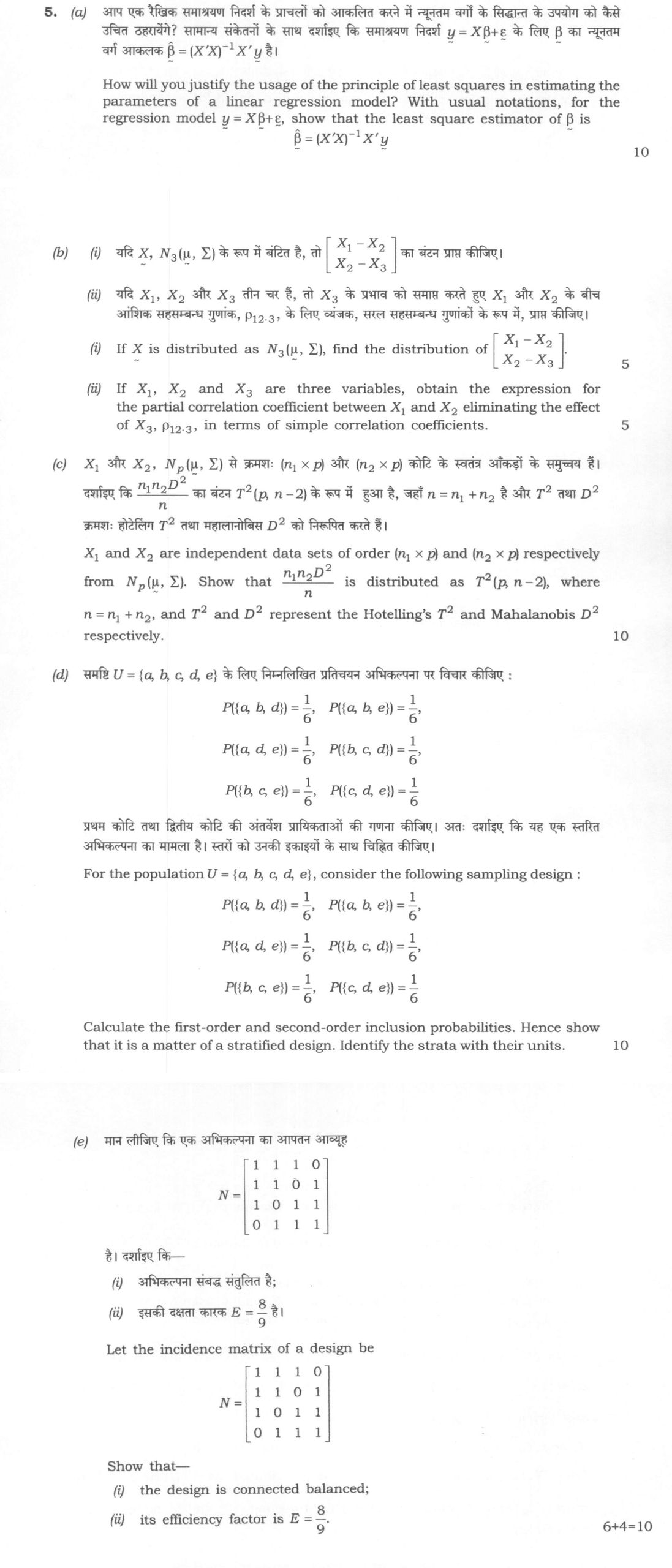
(a) How will you justify the usage of the principle of least squares in estimating the parameters of a linear regression model? With usual notations, for the regression model y = Xβ + ε, show that the least square estimator of β is β̂ = (X'X)⁻¹X'y (1

Question

(a) How will you justify the usage of the principle of least squares in estimating the parameters of a linear regression model? With usual notations, for the regression model y = Xβ + ε, show that the least square estimator of β is β̂ = (X'X)⁻¹X'y (10 marks)

(b) (i) If X̃ is distributed as N₃(μ̃, Σ), find the distribution of [X₁ - X₂; X₂ - X₃]. (5 marks)
(ii) If X₁, X₂ and X₃ are three variables, obtain the expression for the partial correlation coefficient between X₁ and X₂ eliminating the effect of X₃, ρ₁₂·₃, in terms of simple correlation coefficients. (5 marks)

(c) X₁ and X₂ are independent data sets of order (n₁ × p) and (n₂ × p) respectively from Nₚ(μ̃, Σ). Show that (n₁n₂D²)/n is distributed as T²(p, n-2), where n = n₁ + n₂, and T² and D² represent the Hotelling's T² and Mahalanobis D² respectively. (10 marks)

(d) For the population U = {a, b, c, d, e}, consider the following sampling design: P({a, b, d}) = 1/6, P({a, b, e}) = 1/6, P({a, d, e}) = 1/6, P({b, c, d}) = 1/6, P({b, c, e}) = 1/6, P({c, d, e}) = 1/6. Calculate the first-order and second-order inclusion probabilities. Hence show that it is a matter of a stratified design. Identify the strata with their units. (10 marks)

(e) Let the incidence matrix of a design be N = [[1, 1, 1, 0], [1, 1, 0, 1], [1, 0, 1, 1], [0, 1, 1, 1]]. Show that— (i) the design is connected balanced; (ii) its efficiency factor is E = 8/9. (6+4=10 marks)

UPSC Answer Check · Accepted Answer

(a) 
The principle of least squares is justified because it chooses the parameter vector that makes the fitted regression plane closest to the observed data in the Euclidean sense. The residual sum of squares is
RSS(β) = ∑ᵢ (yᵢ - xᵢ'β)² = (y - Xβ)'(y - Xβ).
Minimizing this does not require normality. Under the Gauss-Markov assumptions E(ε)=0, Var(ε)=σ²I, and X full column rank, the least-squares estimator is the best linear unbiased estimator. If ε is normal, it is also the maximum-likelihood estimator. Geometrically, Xβ̂ is the orthogonal projection of y on the column space of X.

Expand RSS:
RSS(β) = y'y - 2β'X'y + β'X'Xβ.
Differentiate with respect to β:
∂RSS/∂β = -2X'y + 2X'Xβ.
The second derivative 2X'X is positive definite when X has full column rank, so the stationary point is a minimum. Set the derivative to zero:
X'Xβ = X'y.
These are the normal equations. If X'X is nonsingular,
β̂ = (X'X)⁻¹X'y.
Condition of validity: X is of full column rank p, so X'X is invertible.

(b)(i) 
Let
Y = [X₁ - X₂; X₂ - X₃] = A X, where A = [[1, -1, 0], [0, 1, -1]].
If X ~ N₃(μ, Σ), then by the affine transformation property of the multivariate normal distribution,
Y ~ N₂(Aμ, AΣA').
Here μ = (μ₁, μ₂, μ₃)'. Thus
E(Y) = (μ₁ - μ₂, μ₂ - μ₃)'.
Let Σ = (σᵢⱼ). Then
Var(X₁ - X₂) = σ₁₁ + σ₂₂ - 2σ₁₂,
Var(X₂ - X₃) = σ₂₂ + σ₃₃ - 2σ₂₃,
Cov(X₁ - X₂, X₂ - X₃) = σ₁₂ - σ₁₃ - σ₂₂ + σ₂₃.
Hence
Y ~ N₂( (μ₁ - μ₂, μ₂ - μ₃)', [[σ₁₁ + σ₂₂ - 2σ₁₂, σ₁₂ - σ₁₃ - σ₂₂ + σ₂₃], [σ₁₂ - σ₁₃ - σ₂₂ + σ₂₃, σ₂₂ + σ₃₃ - 2σ₂₃]] ).

(b)(ii) 
The partial correlation between X₁ and X₂ eliminating X₃ is the correlation between the residuals of X₁ and X₂ after regression on X₃. For the trivariate normal distribution,
Cov(X₁, X₂ | X₃) = σ₁₂ - σ₁₃σ₂₃/σ₃₃,
Var(X₁ | X₃) = σ₁₁ - σ₁₃²/σ₃₃ = σ₁₁(1 - ρ₁₃²),
Var(X₂ | X₃) = σ₂₂ - σ₂₃²/σ₃₃ = σ₂₂(1 - ρ₂₃²).
Therefore
ρ₁₂·₃ = [σ₁₂ - σ₁₃σ₂₃/σ₃₃] / √[(σ₁₁ - σ₁₃²/σ₃₃)(σ₂₂ - σ₂₃²/σ₃₃)].
Divide numerator and denominator by √(σ₁₁σ₂₂). Since ρ₁₂ = σ₁₂/√(σ₁₁σ₂₂), ρ₁₃ = σ₁₃/√(σ₁₁σ₃₃), and ρ₂₃ = σ₂₃/√(σ₂₂σ₃₃),
ρ₁₂·₃ = (ρ₁₂ - ρ₁₃ρ₂₃) / √((1 - ρ₁₃²)(1 - ρ₂₃²)).
This requires |ρ₁₃| < 1 and |ρ₂₃| < 1.

(c) 
Let x̄₁ and x̄₂ be the sample mean vectors of the two independent samples, and let S₁ and S₂ be their sample covariance matrices. Define the pooled covariance matrix
S = [(n₁ - 1)S₁ + (n₂ - 1)S₂]/(n - 2), n = n₁ + n₂.
The Mahalanobis distance is
D² = (x̄₁ - x̄₂)' S⁻¹ (x̄₁ - x̄₂).
We must show that
T² = (n₁n₂/n)D² ~ T²(p, n - 2).

Since the samples are independent and come from Nₚ(μ, Σ),
x̄₁ ~ Nₚ(μ, Σ/n₁), x̄₂ ~ Nₚ(μ, Σ/n₂).
Hence
d = x̄₁ - x̄₂ ~ Nₚ(0, Σ(1/n₁ + 1/n₂)) = Nₚ(0, Σ n/(n₁n₂)).
Let
A = (n₁ - 1)S₁ + (n₂ - 1)S₂.
By the additivity property of Wishart matrices,
A ~ Wₚ(Σ, n - 2),
and A is independent of d. Also S = A/(n - 2).
Now define
y = √(n₁n₂/n) d.
Then y ~ Nₚ(0, Σ). Also
T² = (n₁n₂/n)d'S⁻¹d
= (n₁n₂/n)(n - 2)d'A⁻¹d
= (n - 2)y'A⁻¹y.
By the standard Hotelling T² theorem, if y ~ Nₚ(0, Σ) independently of A ~ Wₚ(Σ, ν), then ν y'A⁻¹y ~ T²(p, ν). Taking ν = n - 2,
 (n₁n₂D²)/n ~ T²(p, n - 2).
This is the central Hotelling T² distribution under equality of the two population mean vectors.

(d) 
The six possible samples, each with probability 1/6, are
S₁ = {a,b,d}, S₂ = {a,b,e}, S₃ = {a,d,e},
S₄ = {b,c,d}, S₅ = {b,c,e}, S₆ = {c,d,e}.
Count appearances of each unit:
a appears in S₁,S₂,S₃, so π(a) = 3/6 = 1/2.
b appears in S₁,S₂,S₄,S₅, so π(b) = 4/6 = 2/3.
c appears in S₄,S₅,S₆, so π(c) = 3/6 = 1/2.
d appears in S₁,S₃,S₄,S₆, so π(d) = 4/6 = 2/3.
e appears in S₂,S₃,S₅,S₆, so π(e) = 4/6 = 2/3.
Thus
π(a)=1/2, π(b)=2/3, π(c)=1/2, π(d)=2/3, π(e)=2/3.

For second-order inclusion probabilities π(ij), count samples containing both i and j:
π(ab)=2/6=1/3, π(ac)=0, π(ad)=2/6=1/3, π(ae)=2/6=1/3,
π(bc)=2/6=1/3, π(bd)=2/6=1/3, π(be)=2/6=1/3,
π(cd)=2/6=1/3, π(ce)=2/6=1/3, π(de)=2/6=1/3.

This is a stratified design with strata
U₁ = {a,c}, sample size 1,
U₂ = {b,d,e}, sample size 2.
Selecting one unit from U₁ and two units from U₂ by simple random sampling without replacement gives six possible samples, each with probability (1/2)(1/3)=1/6. These are exactly S₁ to S₆. Also π(a)=π(c)=1/2; π(b)=π(d)=π(e)=2/3; within U₁, π(ac)=0; within U₂, π(bd)=π(be)=π(de)=1/3; between strata, the product rule gives 1/3.
Hence the design is stratified with strata {a,c} and {b,d,e}.

(e)(i) 
Let rows of N correspond to treatments and columns to blocks. Each row sum is 3, so each treatment occurs r = 3 times. Each column sum is 3, so each block contains k = 3 treatments.
For any two distinct treatments, the number of blocks containing both is the dot product of the corresponding rows. For example,
row₁·row₂ = 1·1 + 1·1 + 1·0 + 0·1 = 2.
Similarly every off-diagonal row dot product equals 2. Thus every pair of treatments occurs together λ = 2 times. Therefore the design is balanced.

Now
N N' = [[3,2,2,2],[2,3,2,2],[2,2,3,2],[2,2,2,3]] = I + 2J.
The C-matrix is
C = rI - (1/k)N N' = 3I - (1/3)(I + 2J)
= (8/3)I - (2/3)J.
For the vector 1, J1 = 4·1, so C1 = (8/3)1 - (2/3)(4·1) = 0.
For any vector v orthogonal to 1, Jv = 0, so Cv = (8/3)v.
Thus C has rank 3 = v - 1, with only one zero eigenvalue corresponding to the overall mean contrast. Hence all treatment contrasts are estimable and the design is connected.
Therefore the design is connected and balanced.

(e)(ii) 
For a balanced incomplete block design, the efficiency factor is
E = λv/(rk).
Here v = 4, r = 3, k = 3, and λ = 2. Hence
E = (2 × 4)/(3 × 3) = 8/9.
Equivalently, the non-zero eigenvalue of C is 8/3, so each canonical efficiency factor is
(8/3)/r = (8/3)/3 = 8/9.
Since all non-zero canonical efficiency factors are equal, their harmonic mean is also 8/9.
Therefore E = 8/9.

(a) How will you justify the usage of the principle of least squares in estimating the parameters of a linear regression model?…

Model answer

What "Derive" is asking you to do

Structure that answers it

Where marks are lost

How this answer will be evaluated

Approach

Key points expected

Evaluation rubric

Must cover

Loses marks

Earns more

Extra mark

Must cover

Loses marks

Earns more

Extra mark

Must cover

Loses marks

Earns more

Extra mark

Must cover

Loses marks

Earns more

Extra mark

Must cover

Loses marks

Earns more

Extra mark

Practice this exact question

More from Statistics 2024 Paper I