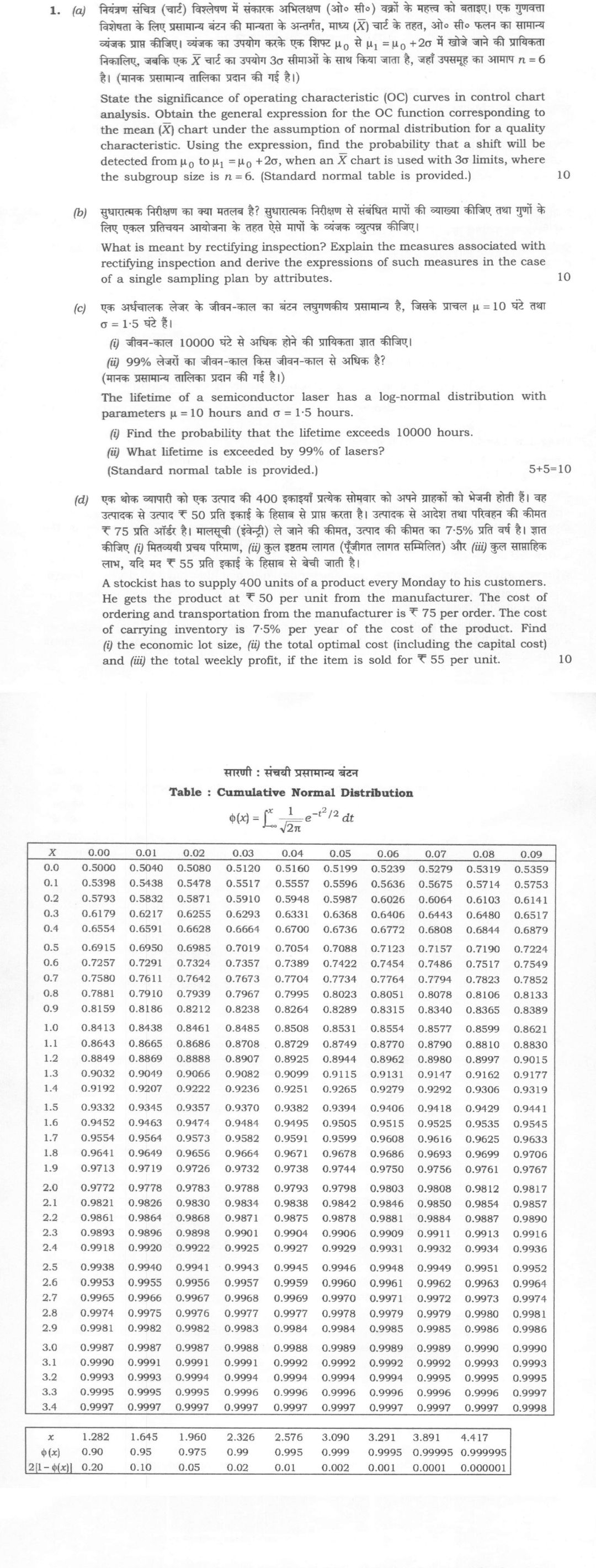
(a) State the significance of operating characteristic (OC) curves in control chart analysis. Obtain the general expression for the OC function corresponding to the mean (X̄) chart under the assumption of normal distribution for a quality characteris

Question

(a) State the significance of operating characteristic (OC) curves in control chart analysis. Obtain the general expression for the OC function corresponding to the mean (X̄) chart under the assumption of normal distribution for a quality characteristic. Using the expression, find the probability that a shift will be detected from μ₀ to μ₁ = μ₀ + 2σ, when an X̄ chart is used with 3σ limits, where the subgroup size is n = 6. (Standard normal table is provided.) 10 marks

(b) What is meant by rectifying inspection? Explain the measures associated with rectifying inspection and derive the expressions of such measures in the case of a single sampling plan by attributes. 10 marks

(c) The lifetime of a semiconductor laser has a log-normal distribution with parameters μ = 10 hours and σ = 1·5 hours.
(i) Find the probability that the lifetime exceeds 10000 hours.
(ii) What lifetime is exceeded by 99% of lasers?
(Standard normal table is provided.) 5+5=10 marks

(d) A stockist has to supply 400 units of a product every Monday to his customers. He gets the product at ₹ 50 per unit from the manufacturer. The cost of ordering and transportation from the manufacturer is ₹ 75 per order. The cost of carrying inventory is 7·5% per year of the cost of the product. Find (i) the economic lot size, (ii) the total optimal cost (including the capital cost) and (iii) the total weekly profit, if the item is sold for ₹ 55 per unit. 10 marks

(e) On the average, 96 patients per 24-hour day require the service of an emergency clinic. Also, on the average, a patient requires 10 minutes of active attention. Assume that the facility can handle only one emergency at a time. Suppose that it costs the clinic ₹ 1,000 per patient treated to obtain an average serving time of 10 minutes, and that each minute of decrease in this average time would cost the clinic ₹ 100 per patient treated. How much would have to be budgeted by the clinic to decrease the average size of the queue from 1 1/3 patients to 1/2 patient? 10 marks

UPSC Answer Check · Accepted Answer

Solve each sub-part systematically with clear problem identification and step-by-step working. For (a), derive the OC function and compute detection probability; for (b), define rectifying inspection and derive AOQ, AOQL, ATI expressions; for (c), apply log-normal transformation and use standard normal tables; for (d), apply EOQ model with all cost components; for (e), use M/M/1 queuing formulas to find service rate changes and budget implications. Allocate approximately 20% time each to parts (a), (b), (c), (d), and (e) respectively, with extra care on derivations in (a) and (b) where method rigor matters most. - (a) Significance of OC curves in assessing Type I/II errors and chart sensitivity; correct derivation of OC function P(|X̄-μ₀|<3σ/√n | μ=μ₁) using normal distribution; calculation of β = P(Z < 1) - P(Z < -5) ≈ 0.1587 for n=6, μ₁-μ₀=2σ - (b) Definition of rectifying inspection as 100% inspection of rejected lots; derivation of AOQ = p·Pa·(N-n)/N, AOQL, and ATI = n·Pa + N(1-Pa) for single sampling plan; explanation of process average quality improvement - (c)(i) Log-normal transformation: ln(10000)=9.2103, Z=(9.2103-10)/1.5=-0.526, P(T>10000)=1-Φ(-0.526)=0.7009 - (c)(ii) Find t where P(T>t)=0.99: Φ⁻¹(0.01)=-2.326, ln(t)=10-3.489=6.511, t=671.5 hours - (d) EOQ calculation: D=400×52=20800, S=75, H=3.75, EOQ=√(2×20800×75/3.75)=912 units; total cost=₹2,08,000+₹17,100+₹17,100=₹2,42,200; weekly profit=400×5-₹4,658=₹1,342 - (e) M/M/1 queue: λ=4/hr, current μ=6/hr (Lq=4²/(6×2)=1.33), target μ=8/hr (Lq=16/32=0.5); budget increase from ₹1,000 to ₹1,200 per patient, total budget ₹1,20,000 for 100 patients/day

Dimension	Weight	Max marks	Excellent	Average	Poor
Setup correctness	20%	10	Correctly identifies all parameters for each sub-part: (a) specifies μ₀, μ₁, σ, n and control limits; (b) defines rectifying inspection with N, n, c, p parameters; (c) recognizes log-normal with μ, σ on log scale; (d) identifies D, S, H correctly with time unit consistency; (e) sets up M/M/1 with λ=4/hr, derives μ from service time	Identifies most parameters but has minor errors like unit inconsistency in (d) or wrong λ conversion in (e), or misses that μ=10 in (c) is log-scale parameter not mean lifetime	Major parameter errors: treats μ=10 in (c) as arithmetic mean, uses wrong time units in (d) or (e), confuses OC curve with ARL, or fails to define rectifying inspection scope
Method choice	20%	10	Selects appropriate methodologies: (a) standardizes using Z=(X̄-μ₁)/(σ/√n) for OC curve; (b) uses hypergeometric/binomial for Pa then derives AOQ/ATI; (c) applies ln transformation for log-normal; (d) uses EOQ formula with annual carrying cost rate; (e) applies Little's formula Lq=λ²/(μ(μ-λ)) for M/M/1	Uses correct broad approach but with shortcuts or omissions, such as approximating binomial with Poisson in (b) without justification, or using wrong queue discipline assumption	Wrong methodology: uses normal directly without log transform in (c), applies P-chart formulas to X̄ chart in (a), uses deterministic EOQ when stochastic needed, or treats (e) as M/D/1 or M/M/c
Computation accuracy	20%	10	Precise calculations with correct standard normal table usage: (a) β=Φ(1)-Φ(-5)=0.8413-0=0.8413, so detection probability=0.1587; (c)(i) Z=-0.5267, area=0.2985, answer=0.7015; (c)(ii) t=exp(6.5108)=671.4 hours; (d) EOQ=912.87, total cost=₹2,42,165; (e) budget=₹1,20,000/day	Generally correct calculations with minor arithmetic errors or table interpolation approximations, such as Z≈-0.53 leading to 0.7019, or rounding EOQ to 900 without recalculating total cost	Significant computational errors: wrong Z-values from tables, arithmetic mistakes in EOQ (e.g., forgetting √), incorrect queue formula application giving negative Lq, or order-of-magnitude errors in (c) due to log scale confusion
Interpretation	20%	10	Clear interpretation of results: (a) explains β as consumer's risk, power=1-β as detection probability; (b) interprets AOQL as worst outgoing quality, ATI as inspection load; (c) notes median lifetime e^μ=22026 hours vs mean; (d) interprets EOQ trade-off and profit margin sensitivity; (e) explains queue reduction cost-effectiveness and service rate investment	States numerical answers with basic interpretation but lacks depth, such as not comparing AOQL to AQL, or failing to note that log-normal is right-skewed making mean > median	No interpretation or incorrect interpretation: treats β as producer's risk, confuses AOQ with AQL, states EOQ without explaining why not exact weekly demand, or gives queue length without operational insight
Final answer & units	20%	10	All answers clearly stated with proper units: (a) probability=0.1587 or 15.87%; (b) AOQ=p·Pa·(N-n)/N, AOQL formula, ATI=n·Pa+N(1-Pa); (c)(i) 0.7015, (c)(ii) 671 hours; (d) EOQ=913 units, total cost=₹2,42,200, weekly profit=₹1,342; (e) ₹1,20,000 per day or ₹4,38,00,000 annually	Most answers present but with inconsistent units (e.g., hours vs years in costs), missing units on probabilities, or unrounded final answers that are hard to interpret	Missing or garbled final answers: no boxed results, confused units (₹ per year vs per week), probability >1 or <0, negative costs, or answers that don't match working

Q1

Directive word: Solve

How this answer will be evaluated

Approach

Key points expected

Evaluation rubric

Practice this exact question

More from Statistics 2025 Paper II