(a) A single-phase AC voltage controller is feeding a resistive load of 26·45 Ω from an AC source of 230 V, 50 Hz. Compute the firing angle to deliver 1000 W to the load. Also compute the p.f. at which this power is delivered. Draw a neat circuit dia

Question

(a) A single-phase AC voltage controller is feeding a resistive load of 26·45 Ω from an AC source of 230 V, 50 Hz. Compute the firing angle to deliver 1000 W to the load. Also compute the p.f. at which this power is delivered. Draw a neat circuit diagram and waveforms of voltage at load terminals with current flowing in the load. 12 marks

(b) An open-loop system G(s) = 1/s²(τs+1) is placed in cascade with a proportional and derivative controller K(s) = (1+Tds). If their unity feedback closed-loop system oscillates at a frequency of √2 rad/second, find the ranges/values of the system and controller parameters, i.e., ranges/values of K, Td and τ. 12 marks

(c) Determine the mechanical time constant of rotor of an electrical machine in terms of its moment of inertia J kg-m² and windage cum friction coefficient f N-m/rad/s. Also explain the method to determine mechanical time constant experimentally in laboratory. 12 marks

(d) An electric train running between two stations A and B, 10 km apart and maintained at voltages 550 V and 500 V respectively, draws a constant current of 600 A. The resistance for both go and return conductors is 0·04 Ω/km. Find the point of minimum potential between the stations, the voltage at that point and currents drawn from both the stations at that point. 12 marks

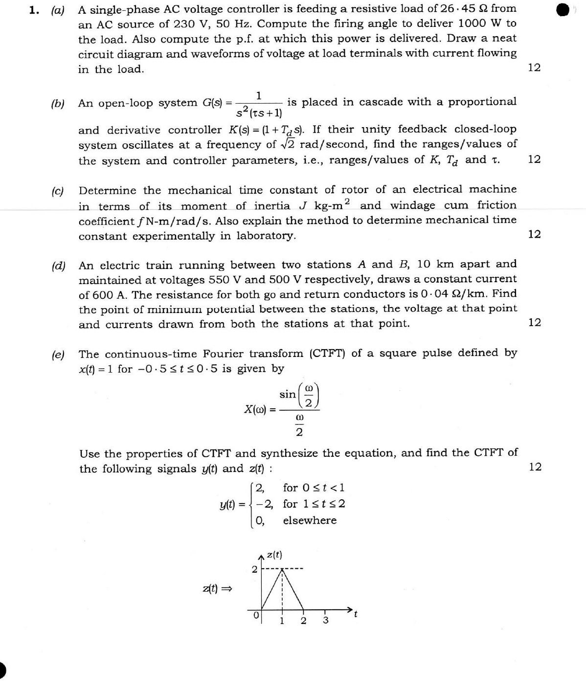
(e) The continuous-time Fourier transform (CTFT) of a square pulse defined by x(t) = 1 for −0·5 ≤ t ≤ 0·5 is given by X(ω) = sin(ω/2)/(ω/2). Use the properties of CTFT and synthesize the equation, and find the CTFT of the following signals y(t) and z(t):
y(t) = {2, for 0 ≤ t < 1; −2, for 1 ≤ t ≤ 2; 0, elsewhere
[diagram of z(t) showing triangular pulse with peak 2 at t=1, zero at t=0 and t=2]
12 marks

UPSC Answer Check · Accepted Answer

Solve all five sub-parts systematically, allocating approximately 20% time to each part given equal 12-mark weighting. Begin with clear circuit diagrams and waveforms for (a), proceed through control system analysis for (b), derive mechanical time constant expression for (c), apply Kirchhoff's laws for traction problem (d), and apply CTFT properties for (e). Present derivations stepwise with final boxed answers for each sub-part.
- Part (a): Correct firing angle calculation using P = (V²/2πR)(2π - α + sin2α/2) = 1000W, yielding α ≈ 90°; power factor = √(P/VA) = √(1000×26.45/230²); circuit diagram showing SCR pair with resistive load; voltage and current waveforms showing conduction from α to π
- Part (b): Characteristic equation 1 + G(s)K(s) = 0 → τs³ + s² + KTd s + K = 0; Routh-Hurwitz criterion application; oscillation condition: auxiliary equation roots at s = ±j√2 yielding K = 2, Td = τ = 1/√2 or equivalent valid ranges
- Part (c): Mechanical time constant τm = J/f seconds; experimental method: run machine at no-load, disconnect supply, measure speed decay time to 36.8% of initial value using tachometer and stopwatch; or use retardation test plotting ω vs t on semilog paper
- Part (d): Set up voltage distribution V(x) = VA - I·r·x - (VA-VB-I·r·L)·x/L for x from A; find dV/dx = 0 for minimum potential point; calculate currents IA and IB using current continuity at minimum potential point
- Part (e): Express y(t) as 2[u(t)-2u(t-1)+u(t-2)] using time-shift and linearity; apply scaling and shifting to get Y(ω) = 2e^(-jω/2)[sin(ω/2)/(ω/2)][1-e^(-jω)]; for z(t) as triangular pulse, use convolution of rectangular pulses or differentiation property

Dimension	Weight	Max marks	Excellent	Average	Poor
Concept correctness	20%	12	Correctly identifies all underlying concepts: RMS voltage control via phase angle in (a), Routh-Hurwitz stability criterion in (b), first-order mechanical system dynamics in (c), distributed parameter traction system in (d), and CTFT properties (time-shifting, scaling, differentiation) in (e); no conceptual errors across any sub-part	Identifies most concepts correctly but has minor errors in one sub-part, such as confusing firing angle control with duty cycle control, or misapplying one CTFT property; understands Routh criterion but makes sign errors	Fundamental conceptual errors in multiple sub-parts, such as treating AC voltage controller as DC chopper, applying wrong stability criterion, or confusing mechanical time constant with electrical time constant
Numerical accuracy	20%	12	All numerical values accurate to appropriate significant figures: firing angle ≈ 90°, pf ≈ 0.707, K=2, Td=τ=1/√2≈0.707s, minimum potential point at 5.5km with 522V, correct CTFT expressions with proper complex coefficients; carries units throughout	Correct approach with minor calculation errors in 1-2 sub-parts, such as arithmetic mistakes in solving transcendental equation or algebraic errors in Routh array; final answers within 10% of correct value	Major numerical errors in multiple sub-parts, missing units, order-of-magnitude mistakes, or incorrect final answers despite correct approach; no verification of reasonableness
Diagram quality	20%	12	Neat, labeled circuit diagram for (a) showing two SCRs in antiparallel with resistive load; clear voltage and current waveforms with firing angle α marked, conduction angles shown; properly sketched z(t) triangular waveform for (e) with peak value 2 and base 0-2s	Diagrams present but lacking clarity: missing labels on axes, unclear marking of firing angle, rough freehand sketches, or waveforms not synchronized properly; z(t) sketch recognizable but dimensions not marked	Missing diagrams for (a), poorly drawn waveforms without proper time/voltage scales, or completely incorrect circuit topology; no attempt at sketching z(t)
Step-by-step derivation	20%	12	Complete stepwise derivations: power integral setup and solution for (a), characteristic equation formation and Routh array construction for (b), torque balance equation leading to τm = J/f for (c), KVL application with distance variable for (d), systematic property application for (e); logical flow with clear justification at each step	Derivations mostly complete but skips key steps or assumes intermediate results without proof; presents final formulas without showing integration limits or Routh array construction; some logical gaps	Missing derivations with only final answers stated, or incorrect derivations with fundamental errors; jumps from given data to conclusion without intermediate steps; no evidence of problem-solving methodology
Practical interpretation	20%	12	Interprets results physically: explains why pf < 1 in (a) due to harmonic content, discusses stability implications of parameter ranges in (b), describes practical measurement precautions for τm in (c), relates minimum potential point to substation spacing in Indian Railways, and explains spectral implications of signal shapes in (e)	Limited physical interpretation; mentions practical relevance superficially without elaboration; may state that results are 'reasonable' without explaining why; standard experimental notes without precautions	No physical interpretation of results; purely mathematical treatment without connecting to real-world implications; ignores practical aspects entirely; no discussion of why answers matter in engineering context

Q1

Directive word: Solve

How this answer will be evaluated

Approach

Key points expected

Evaluation rubric

Practice this exact question

More from Electrical Engineering 2022 Paper II