Paper II — Q8
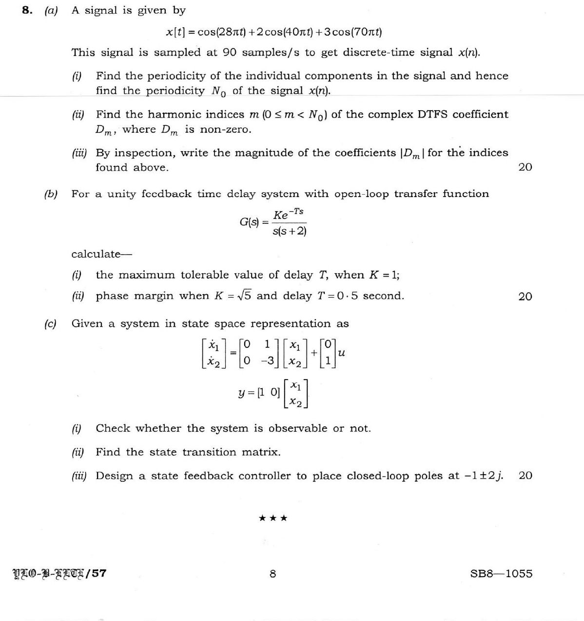
(a) A signal is given by x[t] = cos(28πt) + 2cos(40πt) + 3cos(70πt) This signal is sampled at 90 samples/s to get discrete-time…
A signal is given by
x[t] = cos(28πt) + 2cos(40πt) + 3cos(70πt)
This signal is sampled at 90 samples/s to get discrete-time signal x(n).
Find the periodicity of the individual components in the signal and hence find the periodicity N₀ of the signal x(n).
Find the harmonic indices m (0 ≤ m < N₀) of the complex DTFS coefficient Dₘ, where Dₘ is non-zero.
By inspection, write the magnitude of the coefficients |Dₘ| for the indices found above. 20 marks
For a unity feedback time delay system with open-loop transfer function
G(s) = Ke⁻ᵀˢ/s(s+2)
calculate—
the maximum tolerable value of delay T, when K = 1;
phase margin when K = √5 and delay T = 0·5 second. 20 marks
Given a system in state space representation as
[ẋ₁] [0 1][x₁] [0] [ẋ₂] = [0 -3][x₂] + [1] u
y = [1 0][x₁] [x₂]
Check whether the system is observable or not.
Find the state transition matrix.
Design a state feedback controller to place closed-loop poles at −1±2j. 20 marks
Model answer
Written by UPSC Answer Check against this question's marking rubric, to the expected length. UPSC does not publish answers for Mains — this is one way to score well, not an official key.
(a)(i) The component frequencies are 14 Hz, 20 Hz and 35 Hz, so their continuous periods are 1/14 s, 1/20 s and 1/35 s. With sampling frequency fₛ = 90 samples/s, t = n/90. Hence
x(n) = cos(28πn/90) + 2cos(40πn/90) + 3cos(70πn/90) = cos(14πn/45) + 2cos(4πn/9) + 3cos(7πn/9).
For a discrete component cos(Ωn), period N satisfies ΩN = 2πm, m integer.
- For Ω₁ = 14π/45: (14π/45)N₁ = 2πm ⇒ 7N₁ = 45m ⇒ N₁ = 45.
- For Ω₂ = 4π/9: (4π/9)N₂ = 2πm ⇒ 2N₂ = 9m ⇒ N₂ = 9.
- For Ω₃ = 7π/9: (7π/9)N₃ = 2πm ⇒ 7N₃ = 18m ⇒ N₃ = 18.
Thus N₀ = lcm(45, 9, 18) = 90 samples.
(a)(ii) With N₀ = 90, the DTFS basis is e^(j2πmn/90) = e^(jπmn/45). A cosine A cos(Ωn) contributes at m and at N₀ − m.
- 14πn/45 = π(14)n/45 ⇒ m = 14 and m = 90 − 14 = 76.
- 4πn/9 = 20πn/45 ⇒ m = 20 and m = 70.
- 7πn/9 = 35πn/45 ⇒ m = 35 and m = 55.
Non-zero harmonic indices are m = 14, 20, 35, 55, 70, 76.
(a)(iii) Using A cos(Ωn) = (A/2)e^(jΩn) + (A/2)e^(−jΩn),
- |D₁₄| = 1/2, |D₇₆| = 1/2
- |D₂₀| = 2/2 = 1, |D₇₀| = 1
- |D₃₅| = 3/2, |D₅₅| = 3/2
So the non-zero magnitudes are |D₁₄| = 1/2, |D₂₀| = 1, |D₃₅| = 3/2, |D₅₅| = 3/2, |D₇₀| = 1, |D₇₆| = 1/2.
(b)(i) For G(s) = Ke^(−Ts)/[s(s+2)],
|G(jω)| = K/[ω√(ω² + 4)]
and phase
∠G(jω) = −π/2 − arctan(ω/2) − ωT.
For K = 1, gain crossover is given by
1 = 1/[ω√(ω² + 4)] ⇒ ω²(ω² + 4) = 1.
Let u = ω². Then u² + 4u − 1 = 0, so
u = −2 + √5 = √5 − 2.
Therefore
ω_gc = √(√5 − 2) ≈ 0.485868 rad/s.
Phase margin without delay is
PM = π/2 − arctan(ω_gc/2) = 1.332479 rad.
At marginal stability, PM = ω_gc T_max. Hence
T_max = 1.332479/0.485868 ≈ 2.742 s.
So the maximum tolerable delay is T_max ≈ 2.742 s.
(b)(ii) For K = √5, gain crossover satisfies
√5/[ω√(ω² + 4)] = 1 ⇒ ω²(ω² + 4) = 5.
Let u = ω². Then u² + 4u − 5 = 0 ⇒ u = 1. Thus ω_gc = 1 rad/s.
Phase margin is
PM = π + ∠G(jω_gc)
= π − π/2 − arctan(1/2) − (1)(0.5)
= π/2 − arctan(0.5) − 0.5
= arctan(2) − 0.5 rad
≈ 0.607149 rad
= 34.787°.
(c)(i) A = [0 1; 0 −3], C = [1 0].
Observability matrix:
O = [C; CA] = [[1, 0], [0, 1]].
Since det(O) = 1 ≠ 0 and rank(O) = 2, the system is completely observable.
(c)(ii) The state transition matrix is Φ(t) = e^(At) = L⁻¹[(sI − A)⁻¹].
sI − A = [[s, −1], [0, s + 3]].
Thus
(sI − A)⁻¹ = [[1/s, 1/(s(s+3))], [0, 1/(s+3)]].
Taking inverse Laplace,
Φ(t) = [[1, (1 − e^(−3t))/3], [0, e^(−3t)]], for t ≥ 0.
So
Φ(t) = [[1, (1 − e^(−3t))/3], [0, e^(−3t)]], t ≥ 0.
(c)(iii) Controllability matrix:
[B AB] = [[0, 1], [1, −3]], det = −1 ≠ 0.
So pole placement is possible. Let u = −Kx, where K = [k₁ k₂]. Then
A − BK = [[0, 1], [−k₁, −3 − k₂]].
Characteristic polynomial:
det(sI − (A − BK)) = s² + (3 + k₂)s + k₁.
Desired poles are −1 ± 2j, so desired polynomial is
(s + 1 − 2j)(s + 1 + 2j) = s² + 2s + 5.
Compare:
3 + k₂ = 2 ⇒ k₂ = −1,
k₁ = 5.
Therefore
K = [5, −1], and the control law is u = −5x₁ + x₂.
What "Calculate" is asking you to do
Apply the standard formula or schedule to data the question has already supplied — a table of readings, cost records, a balance sheet — and produce the number. The method is rarely in doubt; the marks sit in the named intermediate quantities, each of which has to appear as a labelled line.
Structure that answers it
Data as given → formula or standard treatment, named → substitution → each intermediate, labelled → result with units
Where marks are lost
Omitting an intermediate the marking scheme pays for separately, or rounding at an intermediate line so the final figure drifts. In commerce and accountancy, any figure in a statement that no numbered working note supports is treated as unearned.
How this answer will be evaluated
Approach
(a(i)) calculate: given > formula > substitution > result with units > interpretation | (a(ii)) calculate: given > formula > substitution > result with units > interpretation | (a(iii)) calculate: given > formula > substitution > result with units > interpretation | (b(i)) calculate: given > formula > substitution > result with units > interpretation | (b(ii)) calculate: given > formula > substitution > result with units > interpretation | (c(i)) calculate: given > formula > substitution > result with units > interpretation | (c(ii)) calculate: given > formula > substitution > result with units > interpretation | (c(iii)) calculate: given > formula > substitution > result with units > interpretation Full marks: All parts solved with correct methods, clear steps, and accurate final values.
Key points expected
- Convert continuous frequencies to discrete-time frequencies
- Calculate period for each cosine component
- Find LCM of individual periods for N0
- Map discrete frequencies to integer indices m
- List all m values for 0 <= m < N0
- Relate time-domain amplitudes to DTFS magnitudes
- List |Dm| for each non-zero index
- Apply Routh-Hurwitz or Nyquist criterion
Evaluation rubric
Each sub-part is marked on its own, against the marks and word limit printed on the paper.
- (a(i)) Determine the period of each component and the fundamental period N0 of the sampled signal.
calculate— given → formula → substitution → result with units → interpretation
Must cover
- Convert continuous frequencies to discrete-time frequencies
- Calculate period for each cosine component
- Find LCM of individual periods for N0
Loses marks
- Confusing continuous time period with discrete time period
- Incorrect LCM calculation
Earns more
- Explicitly states sampling frequency Fs = 90 Hz
- Shows the ratio of discrete to continuous frequency
Extra mark
- Verifies periodicity by checking x(n+N0) = x(n)
- (a(ii)) Identify the specific harmonic indices m where the DTFS coefficients are non-zero.
calculate— given → formula → substitution → result with units → interpretation
Must cover
- Map discrete frequencies to integer indices m
- List all m values for 0 <= m < N0
Loses marks
- Missing negative frequency indices (aliased to positive)
Earns more
- Shows the relationship between frequency and index m
Extra mark
- Notes symmetry of indices for real signals
- (a(iii)) State the magnitude of the DTFS coefficients for the identified indices.
calculate— given → formula → substitution → result with units → interpretation
Must cover
- Relate time-domain amplitudes to DTFS magnitudes
- List |Dm| for each non-zero index
Loses marks
- Forgetting the 1/2 factor for cosine terms
Earns more
- Correctly accounts for the 1/2 factor in cosine expansion
Extra mark
- Mentions phase of coefficients
- (b(i)) Determine the maximum delay T for stability when K=1.
calculate— given → formula → substitution → result with units → interpretation
Must cover
- Apply Routh-Hurwitz or Nyquist criterion
- Solve for the critical value of T
Loses marks
- Ignoring the phase lag of the delay term
Earns more
- Shows the characteristic equation with delay term
Extra mark
- Sketches the Nyquist plot
- (b(ii)) Compute the phase margin for K=sqrt(5) and T=0.5s.
calculate— given → formula → substitution → result with units → interpretation
Must cover
- Find gain crossover frequency
- Calculate phase at crossover frequency
- Compute phase margin
Loses marks
- Incorrect phase calculation for the time delay
Earns more
- Explicitly calculates the phase contribution of the delay
Extra mark
- Verifies stability based on the margin
- (c(i)) Determine if the system is observable using the observability matrix.
calculate— given → formula → substitution → result with units → interpretation
Must cover
- Construct the observability matrix
- Check the rank of the matrix
Loses marks
- Incorrect construction of the observability matrix
Earns more
- States the condition for observability (full rank)
Extra mark
- Uses the PBH test as a check
- (c(ii)) Find the state transition matrix for the given system.
calculate— given → formula → substitution → result with units → interpretation
Must cover
- Compute the matrix exponential e^(At)
- Show the steps for diagonalization or Laplace transform
Loses marks
- Arithmetic errors in matrix inversion or exponentiation
Earns more
- Identifies eigenvalues of the A matrix
Extra mark
- Verifies the result by differentiating
- (c(iii)) Design a state feedback controller to place poles at -1 +/- 2j.
calculate— given → formula → substitution → result with units → interpretation
Must cover
- Form the desired characteristic polynomial
- Equate coefficients to find feedback gain K
- Verify the closed-loop poles
Loses marks
- Incorrect characteristic polynomial for the desired poles
Earns more
- Uses Ackermann's formula or pole placement method
Extra mark
- Sketches the root locus
Practice this exact question
Write your answer and it is marked point by point against the model answer above — what you covered, what you missed, what you got wrong.
Evaluate my answer →More from Electrical Engineering 2022 Paper II
- Q5 (a) A DC motor has an armature resistance of 0·5 Ω and Kφ of 3 Vs. The motor is driven by…
- Q6 (a) A 20 kW, 500 V DC shunt motor (having 90% full-load efficiency) has 40% armature copp…
- Q7 (a) A full-controlled full-wave bridge AC/DC converter is fed from a single-phase, 230 V,…
- Q8 (a) A signal is given by x[t] = cos(28πt) + 2cos(40πt) + 3cos(70πt) This signal is sample…