Paper I — Q8
(a) (i) In stratified sampling under optimum allocation, how will you proceed to select units from different strata, if one or…
In stratified sampling under optimum allocation, how will you proceed to select units from different strata, if one or more nᵢ's happens to be greater than Nᵢ (i ≥ 2) ?
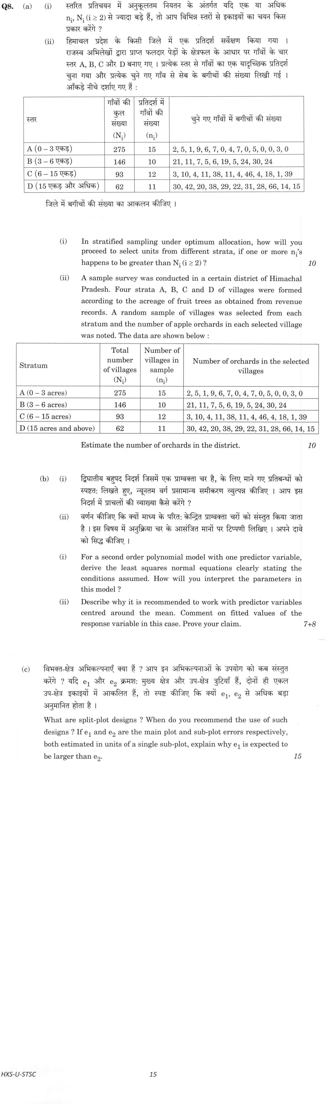
A sample survey was conducted in a certain district of Himachal Pradesh. Four strata A, B, C and D of villages were formed according to the acreage of fruit trees as obtained from revenue records. A random sample of villages was selected from each stratum and the number of apple orchards in each selected village was noted. The data are shown below :
| Stratum | Total number of villages (Nᵢ) | Number of villages in sample (nᵢ) | Number of orchards in the selected villages |
|---|---|---|---|
| A (0 – 3 acres) | 275 | 15 | 2, 5, 1, 9, 6, 7, 0, 4, 7, 0, 5, 0, 0, 3, 0 |
| B (3 – 6 acres) | 146 | 10 | 21, 11, 7, 5, 6, 19, 5, 24, 30, 24 |
| C (6 – 15 acres) | 93 | 12 | 3, 10, 4, 11, 38, 11, 4, 46, 4, 18, 1, 39 |
| D (15 acres and above) | 62 | 11 | 30, 42, 20, 38, 29, 22, 31, 28, 66, 14, 15 |
Estimate the number of orchards in the district.
For a second order polynomial model with one predictor variable, derive the least squares normal equations clearly stating the conditions assumed. How will you interpret the parameters in this model ?
Describe why it is recommended to work with predictor variables centred around the mean. Comment on fitted values of the response variable in this case. Prove your claim.
What are split-plot designs ? When do you recommend the use of such designs ? If e₁ and e₂ are the main plot and sub-plot errors respectively, both estimated in units of a single sub-plot, explain why e₁ is expected to be larger than e₂.
हिंदी में प्रश्न पढ़ें
स्तरीत प्रतिचयन में अनुकूलतम नियतन के अंतर्गत यदि एक या अधिक nᵢ, Nᵢ (i ≥ 2) से ज्यादा बड़े हैं, तो आप विभिन्न स्तरों से इकाइयों का चयन किस प्रकार करेंगे ?
हिमाचल प्रदेश के किसी जिले में एक प्रतिदर्श सर्वेक्षण किया गया । राजस्व अभिलेखों द्वारा प्राप्त फलदार पेड़ों के क्षेत्रफल के आधार पर गाँवों के चार स्तर A, B, C और D बनाए गए । प्रत्येक स्तर से गाँवों का एक यादृच्छिक प्रतिदर्श चुना गया और प्रत्येक चुने गए गाँव से सेब के बगीचों की संख्या लिखी गई । आँकड़े नीचे दर्शाए गए हैं :
| स्तर | गाँवों की कुल संख्या (Nᵢ) | प्रतिदर्श में गाँवों की संख्या (nᵢ) | चुने गए गाँवों में बगीचों की संख्या |
|---|---|---|---|
| A (0 – 3 एकड़) | 275 | 15 | 2, 5, 1, 9, 6, 7, 0, 4, 7, 0, 5, 0, 0, 3, 0 |
| B (3 – 6 एकड़) | 146 | 10 | 21, 11, 7, 5, 6, 19, 5, 24, 30, 24 |
| C (6 – 15 एकड़) | 93 | 12 | 3, 10, 4, 11, 38, 11, 4, 46, 4, 18, 1, 39 |
| D (15 एकड़ और अधिक) | 62 | 11 | 30, 42, 20, 38, 29, 22, 31, 28, 66, 14, 15 |
जिले में बगीचों की संख्या का आकलन कीजिए ।
द्विघातीय बहुपद निर्देश जिसमें एक प्रावकता चर है, के लिए माने गए प्रतिबंधों को स्पष्ट लिखते हुए, न्यूनतम वर्ग प्रसामान्य समीकरण व्युत्पन्न कीजिए । आप इस निर्देश में प्राचलों की व्याख्या कैसे करेंगे ?
वर्णन कीजिए कि क्यों माध्य के परितः केंद्रित प्रावकता चरों को संस्तुत किया जाता है । इस विषय में अनुक्रिया चर के आसंगित मानों पर टिप्पणी लिखिए । अपने दावे को सिद्ध कीजिए ।
विभक्त-क्षेत्र अभिकल्पनाएँ क्या हैं ? आप इन अभिकल्पनाओं के उपयोग को कब संस्तुत करेंगे ? यदि e₁ और e₂ क्रमशः मुख्य क्षेत्र और उप-क्षेत्र त्रुटियाँ हैं, दोनों ही एकल उप-क्षेत्र इकाइयों में आकलित हैं, तो स्पष्ट कीजिए कि क्यों e₁, e₂ से अधिक बड़ा अनुमानित होता है ।
The figure this question refers to, in words
The question paper is a scan and the diagram did not survive as text. This is the figure as read from the original page — every component, value and label — so the question can be worked from the text below.
(a) Table with 4 columns and 4 data rows: Columns: Stratum | Total number of villages (N_i) | Number of villages in sample (n_i) | Number of orchards in the selected villages Row 1: A (0 - 3 acres) | 275 | 15 | 2, 5, 1, 9, 6, 7, 0, 4, 7, 0, 5, 0, 0, 3, 0 Row 2: B (3 - 6 acres) | 146 | 10 | 21, 11, 7, 5, 6, 19, 5, 24, 30, 24 Row 3: C (6 - 15 acres) | 93 | 12 | 3, 10, 4, 11, 38, 11, 4, 46, 4, 18, 1, 39 Row 4: D (15 acres and above) | 62 | 11 | 30, 42, 20, 38, 29, 22, 31, 28, 66, 14, 15
Model answer
Written by UPSC Answer Check against this question's marking rubric, to the expected length. UPSC does not publish answers for Mains — this is one way to score well, not an official key.
(a)(i) Under optimum allocation, first compute the provisional allocation nᵢ = n (NᵢSᵢ)/Σ(NᵢSᵢ), or if costs differ, nᵢ = n (NᵢSᵢ/√Cᵢ)/Σ(NᵢSᵢ/√Cᵢ). If some nᵢ > Nᵢ, that stratum cannot supply more than all its units. Set those nᵢ = Nᵢ and take a complete census in them. Remove these strata from further allocation. Let the remaining sample size be n′ = n − Σ Nᵢ over the exhausted strata. Recompute optimum allocation among the remaining strata using their NᵢSᵢ (or NᵢSᵢ/√Cᵢ). Repeat until every nᵢ ≤ Nᵢ. Finally, select all units in exhausted strata and use SRSWOR with the revised nᵢ in the other strata.
(a)(ii) For stratified random sampling, the unbiased estimate of the population total is Ŷ_st = Σ Nᵢȳᵢ. The stratum totals and means are:
- A: Σy = 49, n = 15, ȳ_A = 49/15, contribution = 275 × 49/15 = 2695/3 = 898.333.
- B: Σy = 152, n = 10, ȳ_B = 152/10 = 15.2, contribution = 146 × 152/10 = 11096/5 = 2219.2.
- C: Σy = 189, n = 12, ȳ_C = 189/12 = 15.75, contribution = 93 × 189/12 = 5859/4 = 1464.75.
- D: Σy = 335, n = 11, ȳ_D = 335/11, contribution = 62 × 335/11 = 20770/11 = 1888.182.
Hence Ŷ_st = 2695/3 + 11096/5 + 5859/4 + 20770/11 = 4270507/660 = 6470.465. Estimated number of orchards in the district ≈ 6470.47, i.e. about 6470 orchards.
(b)(i) Model: yᵢ = β₀ + β₁xᵢ + β₂xᵢ² + εᵢ. Assume xᵢ are fixed, E(εᵢ) = 0, Var(εᵢ) = σ², and εᵢ are uncorrelated. For inference, assume εᵢ are normal. Least squares minimizes Q = Σ(yᵢ − β₀ − β₁xᵢ − β₂xᵢ²)². Differentiating and setting derivatives to zero gives the normal equations:
∂Q/∂β₀ = 0 ⇒ nβ₀ + β₁Σxᵢ + β₂Σxᵢ² = Σyᵢ ∂Q/∂β₁ = 0 ⇒ β₀Σxᵢ + β₁Σxᵢ² + β₂Σxᵢ³ = Σxᵢyᵢ ∂Q/∂β₂ = 0 ⇒ β₀Σxᵢ² + β₁Σxᵢ³ + β₂Σxᵢ⁴ = Σxᵢ²yᵢ.
In matrix form, X′Xβ = X′y, where X = [1, x, x²].
Interpretation: β₀ is the expected response at x = 0, if x = 0 is meaningful. β₁ is the slope of the curve at x = 0, since dy/dx = β₁ + 2β₂x. β₂ measures curvature; β₂ > 0 gives upward curvature, β₂ < 0 gives downward curvature. The turning point is x* = −β₁/(2β₂).
(b)(ii) Centring replaces xᵢ by zᵢ = xᵢ − x̄. The model becomes y = γ₀ + γ₁z + γ₂z² + ε. This is recommended because x and x² are often highly correlated when x is far from zero. Centring makes Σz = 0, reduces non-essential ill-conditioning, improves numerical stability, and makes γ₀ the expected response at the mean predictor x̄.
The fitted values are unchanged. Since 1 = 1, z = x − x̄, z² = x² − 2x̄x + x̄², the column space of [1, z, z²] is exactly the same as that of [1, x, x²]. Hence the least-squares projection matrix is the same, so ŷᵢ = β̂₀ + β̂₁xᵢ + β̂₂xᵢ² = γ̂₀ + γ̂₁zᵢ + γ̂₂zᵢ². The coefficients transform as β₂ = γ₂, β₁ = γ₁ − 2γ₂x̄, β₀ = γ₀ − γ₁x̄ + γ₂x̄². The residuals and SSE remain identical. The centred intercept γ̂₀ is the fitted value at x = x̄.
(c) A split-plot design is a two-stage factorial design. Whole plots, also called main plots, receive one set of treatments, usually the factor that is difficult or costly to change. Each whole plot is then divided into sub-plots, and the second factor is randomized to sub-plots within each whole plot. Thus randomization is done at two levels.
It is recommended when one factor requires large experimental units or is hard to change, while another factor can be applied to smaller units; when a natural hierarchy of experimental units exists; and when greater precision is wanted for the sub-plot factor and its interaction with the whole-plot factor.
In the model y = μ + main-plot effects + e₁ + sub-plot effects + e₂, e₁ is the main-plot error and e₂ is the sub-plot error. The main-plot error measures variation among whole plots after accounting for main-plot treatments. The sub-plot error measures variation among sub-plots within the same whole plot. Since whole plots are larger and more heterogeneous, and e₁ contains the extra whole-plot variation in addition to the sub-plot variation, e₁ is expected to be larger than e₂. Therefore comparisons of main-plot treatments are less precise, while sub-plot treatment comparisons are more precise.
What "Solve" is asking you to do
Choose the method, then carry it through to a final answer. Identifying what kind of problem this is and why that method applies is the first thing marked; a correct figure arrived at invisibly earns almost nothing.
Structure that answers it
Given data and what is required → method chosen, with the reason it applies → set-up (equation, circuit, free body, trial balance) → working, step by step → answer with units and any condition of validity
Where marks are lost
Doing the middle steps mentally and writing only the result. In mathematics papers, a further loss comes from giving a decimal where the exact value in surds or fractions was wanted, or from skipping the justification a part explicitly asks for.
How this answer will be evaluated
Approach
Framework: UPSC Statistics Paper 1. (a(i)) explain: definition/context > points in order > small example > short close | (a(ii)) calculate: given > formula > substitution > result with units > interpretation | (b(i)) derive: given > assumptions > stepwise derivation > result > check | (b(ii)) describe: define > structure or process in order > labelled diagram > significance | (c) explain: definition/context > points in order > small example > short close Full marks: Complete derivations with correct notation, accurate calculations, clear interpretations, and proper statistical reasoning throughout.
Key points expected
- Identify strata where n_i > N_i
- Specify use of census for those strata
- Adjust allocation for remaining strata
- Calculate sample mean for each stratum
- Apply stratified estimator formula
- Sum weighted stratum estimates
- State final estimate clearly
- State model y = β0 + β1x + β2x² + ε
Evaluation rubric
Each sub-part is marked on its own, against the marks and word limit printed on the paper.
- (a(i)) Procedure for handling n_i > N_i in optimum allocation.
explain— definition/context → points in order → small example → short close
Must cover
- Identify strata where n_i > N_i
- Specify use of census for those strata
- Adjust allocation for remaining strata
Loses marks
- Ignoring the condition n_i > N_i
- Treating all strata identically
Earns more
- Mentioning Neyman allocation formula
- Discussing variance implications
Extra mark
- Citing specific sampling theory text
- (a(ii)) Estimate total number of orchards in the district. 10 marks
calculate— given → formula → substitution → result with units → interpretation
Must cover
- Calculate sample mean for each stratum
- Apply stratified estimator formula
- Sum weighted stratum estimates
- State final estimate clearly
Loses marks
- Arithmetic errors in means
- Omitting stratum weights
Earns more
- Showing intermediate calculations
- Using correct notation for N_i and n_i
Extra mark
- Calculating standard error of estimate
- (b(i)) Derive least squares normal equations for quadratic model.
derive— given → assumptions → stepwise derivation → result → check
Must cover
- State model y = β0 + β1x + β2x² + ε
- Write sum of squared errors function
- Differentiate w.r.t. each β
- Present resulting normal equations
Loses marks
- Incorrect differentiation
- Missing terms in equations
Earns more
- Stating assumptions of OLS
- Interpreting β0, β1, β2 parameters
Extra mark
- Matrix form of normal equations
- (b(ii)) Explain benefits of centering predictor variables. 15 marks
describe— define → structure or process in order → labelled diagram → significance
Must cover
- Define centering transformation
- Explain reduction in multicollinearity
- Discuss interpretation of intercept
- Prove claim with mathematical argument
Loses marks
- Vague explanation without proof
- Confusing centering with scaling
Earns more
- Showing correlation matrix before/after
- Discussing numerical stability
Extra mark
- Example with actual data
- (c) Define split-plot designs and explain error structure. 15 marks
explain— definition/context → points in order → small example → short close
Must cover
- Define split-plot design structure
- Identify when to use such designs
- Explain main plot vs sub-plot errors
- Justify why e1 > e2
Loses marks
- Confusing with factorial designs
- Incorrect error term assignment
Earns more
- Diagram of split-plot layout
- Example of agricultural application
Extra mark
- ANOVA table for split-plot
Practice this exact question
Write your answer and it is marked point by point against the model answer above — what you covered, what you missed, what you got wrong.
Evaluate my answer →More from Statistics 2021 Paper I
- Q5 (a) For a simple linear regression model Y = β₀ + β₁Xᵢ + εᵢ, i = 1, ..., n (i) Derive the…
- Q6 (a) For a multiple linear regression model with three covariates X₁, X₂ and X₃, let rᵢⱼ d…
- Q7 (a) (i) What is confounding in factorial experiments ? (ii) A 2^6factorial experiment is…
- Q8 (a) (i) In stratified sampling under optimum allocation, how will you proceed to select u…