Paper II — Q1
Explain Single Sampling Plan with the help of an example. Also, write the importance of an Operating Characteristics Curve in a…
Explain Single Sampling Plan with the help of an example. Also, write the importance of an Operating Characteristics Curve in a sampling plan. 10 marks
Solve the above assignment problem.
Depot I II III IV V A 160 130 175 190 200 Town B 135 120 130 160 175 C 140 110 145 170 185 D 50 50 80 80 110 E 55 35 80 80 105 10 marks
Use algebraic method to solve the above game.
Player B B₁ B₂ B₃ B₄ A₁ 0·25 0·20 0·14 0·30 Player A A₂ 0·27 0·16 0·12 0·14 A₃ 0·35 0·08 0·15 0·19 A₄ −0·02 0·08 0·13 0·00 10 marks
Consider the Markov Chain with transition probability matrix:
0 1 2 0 (0 1 0) 1 (½ 0 ½) 2 (0 1 0)
Show that the states are periodic and persistent non-null. 10 marks
State the importance of the hazard function. If the hazard rate of a component is given by:
h(t) = { 0.015, t ≤ 200 { 0.025, t > 200
then find an expression for the reliability function of the component. 10 marks
हिंदी में प्रश्न पढ़ें
एक उदाहरण की सहायता से, एकल प्रतिचयन आयोजना की व्याख्या कीजिए। एक प्रतिचयन आयोजना में संकारक अभिलक्षण वक्र के महत्व को भी लिखिए। (10 अंक)
निम्नलिखित नियतन समस्या को हल कीजिए :
डिपो I II III IV V A 160 130 175 190 200 शहर B 135 120 130 160 175 C 140 110 145 170 185 D 50 50 80 80 110 E 55 35 80 80 105 (10 अंक)
बीजीय विधि का उपयोग करके निम्नलिखित खेल को हल कीजिए :
खिलाड़ी B B₁ B₂ B₃ B₄ A₁ 0·25 0·20 0·14 0·30 खिलाड़ी A A₂ 0·27 0·16 0·12 0·14 A₃ 0·35 0·08 0·15 0·19 A₄ −0·02 0·08 0·13 0·00 (10 अंक)
संक्रमण प्रायिकता आव्यूह
0 1 2 0 (0 1 0) 1 (½ 0 ½) 2 (0 1 0)
के साथ एक मार्कोव श्रृंखला पर विचार कीजिए। दर्शाइए कि अवस्थाएँ आवर्ती और सततावृत अनिराकरणीय हैं। (10 अंक)
संकटप्रस्तता फलन के महत्व को बताइए। यदि किसी घटक की संकटप्रस्तता दर इस प्रकार दी गई है :
h(t) = { 0.015, t ≤ 200 { 0.025, t > 200
तो घटक के विश्वसनीयता फलन के एक व्यंजक को प्राप्त कीजिए। (10 अंक)
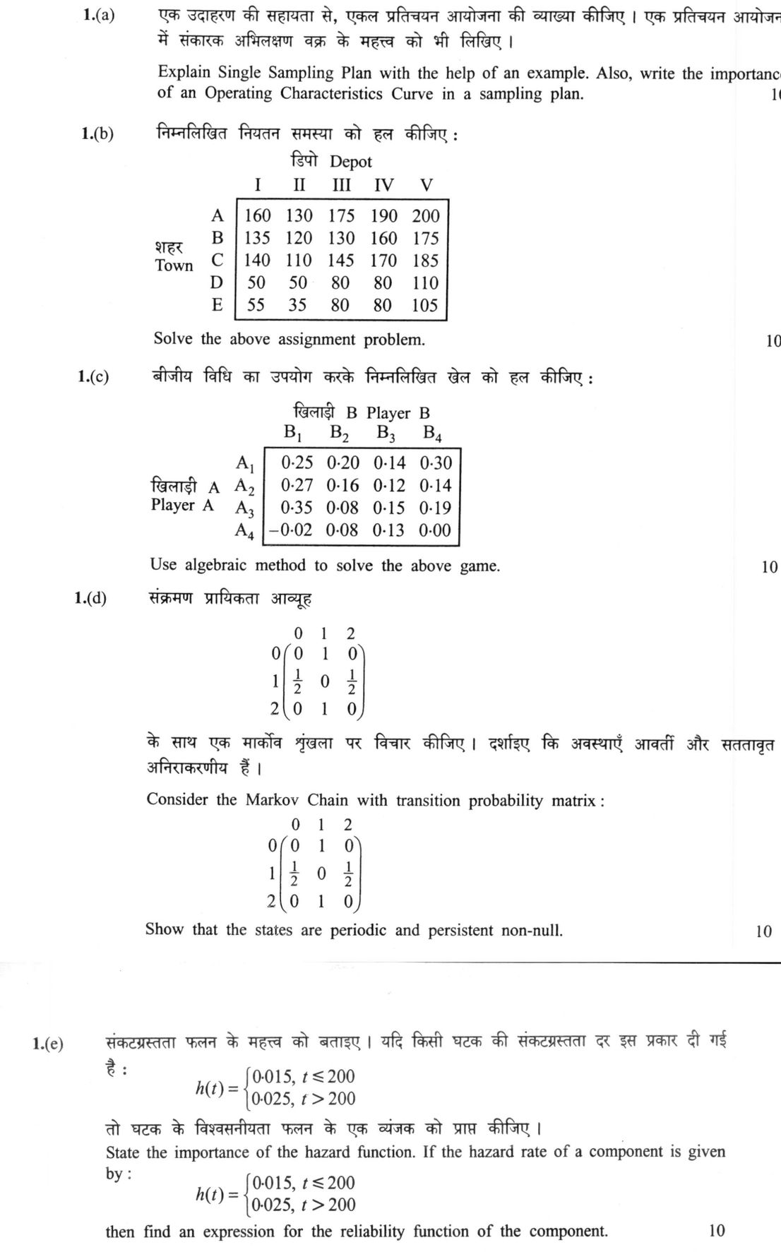
The figure this question refers to, in words
The question paper is a scan and the diagram did not survive as text. This is the figure as read from the original page — every component, value and label — so the question can be worked from the text below.
(b) Depot: I, II, III, IV, V Town A: 160, 130, 175, 190, 200 Town B: 135, 120, 130, 160, 175 Town C: 140, 110, 145, 170, 185 Town D: 50, 50, 80, 80, 110 Town E: 55, 35, 80, 80, 105
(c) Player B: B1, B2, B3, B4 Player A A1: 0.25, 0.20, 0.14, 0.30 Player A A2: 0.27, 0.16, 0.12, 0.14 Player A A3: 0.35, 0.08, 0.15, 0.19 Player A A4: -0.02, 0.08, 0.13, 0.00
Model answer
Written by UPSC Answer Check against this question's marking rubric, to the expected length. UPSC does not publish answers for Mains — this is one way to score well, not an official key.
(a) Single Sampling Plan A single sampling plan is defined by the lot size N, sample size n, and acceptance number c. Draw a random sample of n items from the lot and count defectives d. If d ≤ c, accept the lot; if d > c, reject it. Example: N = 1000, n = 50, c = 1. Accept if 0 or 1 defective is found; reject if 2 or more defectives are found. If the lot fraction defective is p, then Pa(p) = Σ₍d=0₎¹ C(50,d) p^d (1−p)^(50−d) = (1−p)^50 + 50p(1−p)^49. At p = 0.01, Pa ≈ 0.91; at p = 0.05, Pa ≈ 0.28. The Operating Characteristics curve plots Pa(p) against p. Its importance is that it measures the discriminating power of the plan, shows producer’s risk α and consumer’s risk β, helps fix AQL and LTPD, compares alternative plans, and guides choice of n and c balancing inspection cost and quality protection.
(b) Assignment Problem Assuming costs are to be minimised. The cost matrix is:
A: 160, 130, 175, 190, 200 B: 135, 120, 130, 160, 175 C: 140, 110, 145, 170, 185 D: 50, 50, 80, 80, 110 E: 55, 35, 80, 80, 105
Row minima are 130, 120, 110, 50, 35. Subtract them. Column minima after row reduction are 0, 0, 10, 30, 55. Subtract them. Cover all zeros by rows B, D and column II; the smallest uncovered entry is 15. Subtract 15 from uncovered entries and add 15 at intersections BII and DII. A zero matching is then: A→V, B→III, C→II, D→I, E→IV. Total minimum cost = 200 + 130 + 110 + 50 + 80 = 570 cost units.
(c) Game The payoff matrix is to Player A. A₃ dominates A₄, so delete A₄. Then B₂ dominates B₁ and B₃ dominates B₄; delete B₁ and B₄. In the remaining matrix, A₁ dominates A₂. The reduced 2×2 game is: A₁: 0.20, 0.14 A₃: 0.08, 0.15
Let A play A₁ with probability p and A₃ with 1−p. For B₂ and B₃ payoffs to be equal: 0.20p + 0.08(1−p) = 0.14p + 0.15(1−p) ⇒ 0.08 + 0.12p = 0.15 − 0.01p ⇒ 0.13p = 0.07 ⇒ p = 7/13, 1−p = 6/13. Let B play B₂ with probability q and B₃ with 1−q. Equating A₁ and A₃ payoffs: 0.20q + 0.14(1−q) = 0.08q + 0.15(1−q) ⇒ 0.14 + 0.06q = 0.15 − 0.07q ⇒ 0.13q = 0.01 ⇒ q = 1/13, 1−q = 12/13. Value v = 0.14 + 0.06(1/13) = 47/325 ≈ 0.1446. Optimal strategies: A: (7/13, 0, 6/13, 0); B: (0, 1/13, 12/13, 0). Value of game to A = 47/325.
(d) Markov Chain The transition matrix is 0: (0, 1, 0) 1: (½, 0, ½) 2: (0, 1, 0) Every transition goes from {0,2} to {1} or from {1} to {0,2}. Hence a return to any state is possible only in an even number of steps. Also two-step returns are positive, e.g. 0→1→0, 1→0→1 or 1→2→1, 2→1→2. Thus every state has period 2. The chain is irreducible because 0↔1↔2. A finite irreducible chain is persistent. For non-null, solve πP = π: π₀ = ½π₁, π₁ = π₀ + π₂, π₂ = ½π₁, π₀ + π₁ + π₂ = 1. This gives π = (¼, ½, ¼). Since the stationary distribution is positive, all states are persistent non-null.
(e)(i) Importance of Hazard Function The hazard function is h(t) = f(t)/R(t). It gives the instantaneous failure rate at time t given survival up to t. It is important because it describes ageing or wear-out behaviour, distinguishes increasing/decreasing/constant failure rates, helps derive R(t) = exp(−∫₀^t h(u)du), and is used in reliability, survival analysis and maintenance decisions.
(e)(ii) Reliability Function R(t) = exp(−∫₀^t h(u)du). For 0 ≤ t ≤ 200: R(t) = exp(−∫₀^t 0.015 du) = e^(−0.015t). For t > 200: ∫₀^t h(u)du = ∫₀^200 0.015 du + ∫₂₀₀^t 0.025 du = 3 + 0.025(t−200) = 0.025t − 2. Hence R(t) = e^(−(0.025t−2)) = e^(2−0.025t). Therefore, R(t) = e^(−0.015t) for 0 ≤ t ≤ 200, and R(t) = e^(2−0.025t) for t > 200, with t in the same time unit as the hazard rate.
What "Solve" is asking you to do
Choose the method, then carry it through to a final answer. Identifying what kind of problem this is and why that method applies is the first thing marked; a correct figure arrived at invisibly earns almost nothing.
Structure that answers it
Given data and what is required → method chosen, with the reason it applies → set-up (equation, circuit, free body, trial balance) → working, step by step → answer with units and any condition of validity
Where marks are lost
Doing the middle steps mentally and writing only the result. In mathematics papers, a further loss comes from giving a decimal where the exact value in surds or fractions was wanted, or from skipping the justification a part explicitly asks for.
How this answer will be evaluated
Approach
(1(a)) explain: definition/context > points in order > small example > short close | (1(b)) calculate: given > formula > substitution > result with units > interpretation | (1(c)) calculate: given > formula > substitution > result with units > interpretation | (1(d)) justify: claim > 3-4 reasons > evidence > conclusion | (1(e)) calculate: given > formula > substitution > result with units > interpretation Full marks: Rigorous derivations, correct algebraic solutions, and clear interpretation of statistical concepts.
Key points expected
- Define Single Sampling Plan (n, c, N)
- Provide a numerical example with n and c
- Define Operating Characteristic (OC) curve
- Explain importance of OC curve (producer/consumer risk)
- Apply Hungarian method (row/column reduction)
- Show initial and final allocation table
- Calculate total minimum cost
- Verify optimality (e.g., opportunity costs)
Evaluation rubric
Each sub-part is marked on its own, against the marks and word limit printed on the paper.
- (1(a)) Definition of Single Sampling Plan, a worked example, and the role of the OC curve. 10 marks
explain— definition/context → points in order → small example → short close
Must cover
- Define Single Sampling Plan (n, c, N)
- Provide a numerical example with n and c
- Define Operating Characteristic (OC) curve
- Explain importance of OC curve (producer/consumer risk)
Loses marks
- Confusing single with double sampling
- No example provided
- OC curve importance not linked to decision making
Earns more
- Mention Producer's Risk (alpha)
- Mention Consumer's Risk (beta)
- Sketch or describe shape of OC curve
Extra mark
- Reference to AQL or LTPD
- (1(b)) Optimal assignment and minimum cost for the 5x5 transportation matrix. 10 marks
calculate— given → formula → substitution → result with units → interpretation
Must cover
- Apply Hungarian method (row/column reduction)
- Show initial and final allocation table
- Calculate total minimum cost
- Verify optimality (e.g., opportunity costs)
Loses marks
- Arithmetic errors in reduction
- Invalid assignment (row/col conflict)
- No final cost calculation
Earns more
- Correct row reduction steps
- Correct column reduction steps
- Clear final assignment list (A-I, B-II, etc.)
Extra mark
- Alternative optimal solution identified
- (1(c)) Optimal mixed strategies and value of the game using algebraic method. 10 marks
calculate— given → formula → substitution → result with units → interpretation
Must cover
- Identify saddle point (or lack thereof)
- Set up algebraic equations for probabilities
- Solve for Player A's strategy (p1, p2...)
- Solve for Player B's strategy (q1, q2...)
Loses marks
- Using graphical method instead of algebraic
- Incorrect setup of expected value equations
- Probabilities not summing to 1
Earns more
- Correct calculation of game value (V)
- Verification that V is consistent for both players
- Clear statement of optimal strategies
Extra mark
- Check for dominated strategies before solving
- (1(d)) Proof that states 0, 1, 2 are periodic and persistent non-null. 10 marks
justify— claim → 3-4 reasons → evidence → conclusion
Must cover
- Define periodicity (period d > 1)
- Show return probabilities for state 0 (e.g., P00(2)>0)
- Define persistent (recurrent) state
- Show sum of return probabilities is 1
Loses marks
- Confusing periodic with transient
- Failing to show d=2 for all states
- No proof of persistence (sum of probabilities)
Earns more
- Calculate P00(2n) and P00(2n+1)
- Demonstrate non-null (finite mean return time)
- Use transition matrix powers explicitly
Extra mark
- Mention irreducibility of the chain
- (1(e)) Importance of hazard function and derivation of reliability function R(t). 10 marks
calculate— given → formula → substitution → result with units → interpretation
Must cover
- State importance of hazard function (failure rate)
- Use formula R(t) = exp(-integral h(t) dt)
- Calculate integral for t <= 200
- Calculate integral for t > 200 (piecewise)
Loses marks
- Ignoring the piecewise nature of h(t)
- Incorrect integration limits
- Missing the negative sign in exponent
Earns more
- Correct integration of constant h(t)
- Correct handling of the discontinuity at t=200
- Final expression for R(t) in piecewise form
Extra mark
- Interpretation of R(200) value
Practice this exact question
Write your answer and it is marked point by point against the model answer above — what you covered, what you missed, what you got wrong.
Evaluate my answer →More from Statistics 2021 Paper II
- Q1 Explain Single Sampling Plan with the help of an example. Also, write the importance of a…
- Q2 A manufacturer finds that on the average, a television set is used 1.8 hours per day. A o…
- Q3 (a) Explain M|G|1 queuing system. Obtain Pollaczek-kinchine formula. (15 marks) (b) Use M…
- Q4 (a) Solve the following linear programming problem: Maximize z = 3x₁ + 5x₂ subject to the…