(a) Consider Poisson distribution

P_θ(X = j) = (e⁻θ θ^j)/(j!) = pⱼ, j = 0, 1, 2, ....

Let fⱼ be the frequency for X = j and E(fⱼ) = mⱼ = npⱼ. Discuss how you obtain minimum chi-square estimate for θ. Does minimum chi-square method necessarily yield

Question

(a) Consider Poisson distribution

P_θ(X = j) = (e⁻θ θ^j)/(j!) = pⱼ, j = 0, 1, 2, ....

Let fⱼ be the frequency for X = j and E(fⱼ) = mⱼ = npⱼ. Discuss how you obtain minimum chi-square estimate for θ. Does minimum chi-square method necessarily yield a sufficient statistic even if it exists ? (20 marks)

(b) (i) Let the joint probability density function of X and Y be

f(x, y) = C . exp -(4x² + 9y² - xy),

where C is a constant. Find E(X), V(X), E(Y), V(Y) and the correlation coefficient between X and Y. (10 marks)

(ii) If X₁, X₂, ..., X₆ are independent random variables such that

P(Xᵢ = -1) = P(Xᵢ = 1) = 1/2, i = 1, 2, ..., 6,

then obtain the value of

P[Σᵢ₌₁⁶ Xᵢ = 4]. (5 marks)

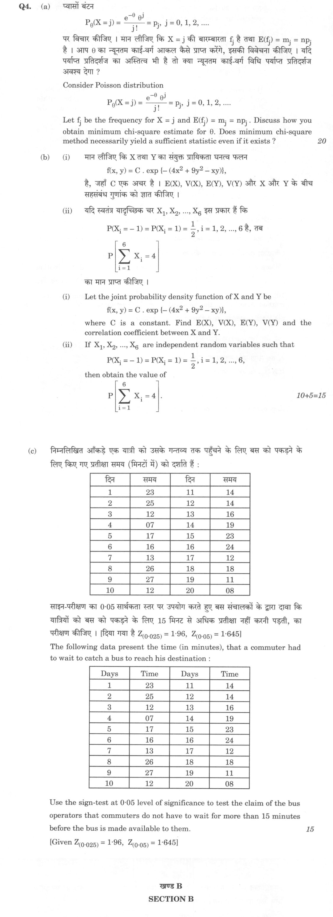
(c) The following data present the time (in minutes), that a commuter had to wait to catch a bus to reach his destination :

Use the sign-test at 0·05 level of significance to test the claim of the bus operators that commuters do not have to wait for more than 15 minutes before the bus is made available to them.

[Given Z₍₀.₀₂₅₎ = 1·96, Z₍₀.₀₅₎ = 1·645] (15 marks)

UPSC Answer Check · Accepted Answer

(a) Minimum chi-square estimate. In minimum chi-square estimation, the observed frequencies fⱼ are compared with the expected frequencies mⱼ=npⱼ(θ), and one minimizes the Pearson statistic
Q(θ)=Σⱼ ((fⱼ-npⱼ)²)/(npⱼ)
over θ>0. Since Σⱼ fⱼ=n and Σⱼ pⱼ=1, the statistic can be written as
Q(θ)=Σⱼ (fⱼ²)/(npⱼ)-n;
the constant -n does not affect the minimization. Differentiating with respect to θ gives
dQ/(dθ)=-Σⱼ (fⱼ² pⱼ'(θ))/(n pⱼ²(θ)),
so the minimum chi-square estimate hatθ is obtained from the estimating equation
Σⱼ (fⱼ² pⱼ'(θ))/(pⱼ²(θ))=0.
For the Poisson distribution, pⱼ(θ)=e⁻θθ^j/j!, so pⱼ'/pⱼ=j/θ-1. Substitution gives
Σⱼ (fⱼ²(j/θ-1))/(pⱼ(θ))=0,
equivalently
θ=(Σⱼ j fⱼ²/pⱼ(θ))/(Σⱼ fⱼ²/pⱼ(θ)).
This equation is implicit because pⱼ depends on θ; it is normally solved by iteration, starting for example from the method-of-moments value θ=Σⱼ j fⱼ/n. The infinite Poisson tail is first grouped so that expected cell frequencies are not too small, and the iteration is repeated until convergence. The solution is checked as a minimum by the second derivative or by comparing Q at nearby values; θ must remain positive.

The minimum chi-square method does not necessarily produce a sufficient statistic. For a Poisson sample, the likelihood factorizes through T=Σ xᵢ, so the sample mean is sufficient, and it is also the MLE. The MCS estimator, however, is a function of the frequency table and generally differs from the sample mean; it gives weight fⱼ² to each cell and therefore depends on the dispersion of the observed counts, not merely on their total. If the data are grouped, the estimator is a function of grouped counts and cannot retain all information about θ. For example, grouping a Poisson sample into 0,1,2 and 3+ gives an MCS estimate based on four grouped counts, while the sufficient statistic is the ungrouped total; different samples with the same total can give different grouped MCS estimates. Thus, even when an MCS estimator exists, sufficiency is not guaranteed; sufficiency is a property of the statistic and the model, not of the minimum chi-square criterion.

(b)(i) The given density is of bivariate normal form. The exponent has no linear terms, so the means are zero. Completing the quadratic form,
exp[-(4x²+9y²-xy)]=exp[-frac12(8x²-2xy+18y²)].
Hence the precision matrix is
8&-1
-1&18.
Its inverse is the covariance matrix:
1/(8·18-1²)
18&1
1&8
=
frac1143
18&1
1&8.
The normalizing constant is C=√143/(2π), though it is not needed for the moments. Therefore
E(X)=0, E(Y)=0, V(X)=18/143, V(Y)=8/143, Cov(X,Y)=frac1143.
The correlation coefficient is
ρ=(Cov(X,Y))/(√(V(X)V(Y)))
=(1/143)/(√((18/143)(8/143)))=frac112.
Thus X and Y are positively but weakly correlated.

(b)(ii) Let N be the number of variables equal to +1. Then NsimBinomial(6,1/2), and
Σᵢ₌₁⁶ Xᵢ=N-(6-N)=2N-6.
The event Σ Xᵢ=4 requires 2N-6=4, so N=5. Hence
P(Σᵢ₌₁⁶ Xᵢ=4)=binom65(frac12)⁶=frac664=frac332.

(c) The twenty waiting times are 23, 25, 12, 7, 17, 16, 13, 26, 27, 12, 14, 14, 16, 19, 23, 24, 12, 18, 11, 8. The operators’ claim that commuters do not wait more than 15 minutes is tested as H₀: median ≤ 15 against H₁: median >15. In the sign test, observations equal to 15 are discarded; here none occur. The positive signs, i.e. waits above 15, are 23, 25, 17, 16, 26, 27, 16, 19, 23, 24 and 18, giving b=11. The negative signs are 12, 7, 13, 12, 14, 14, 12, 11, 8, so n-b=9. Under H₀, B, the number of positive signs, has a Binomial(20,1/2) distribution. The sign test is non-parametric and does not assume normality of waiting times. For a one-sided test at 0.05, use the normal approximation with continuity correction:
Z=(b-0.5-n/2)/(√(n/4))
=(11-0.5-10)/(sqrt5)
=0.5/2.236=0.224.
The supplied 1.96 is for a two-sided 5% test; here the alternative is one-sided, so Z₀.05=1.645 is the relevant critical value. Since 0.224<1.645, we do not reject H₀. The exact binomial one-sided p-value is P(B≥11)=0.412, agreeing with the normal approximation. The data do not provide statistically significant evidence that the median waiting time exceeds 15 minutes; the operators’ claim is not contradicted by this sample.

(a) Consider Poisson distribution P_θ(X = j) = (e⁻θ θ^j)/(j!) = pⱼ, j = 0, 1, 2, .... Let fⱼ be the frequency for X = j and…

The figure this question refers to, in words

Model answer

What "Discuss" is asking you to do

Structure that answers it

Where marks are lost

How this answer will be evaluated

Approach

Key points expected

Evaluation rubric

Must cover

Loses marks

Earns more

Extra mark

Must cover

Loses marks

Earns more

Extra mark

Must cover

Loses marks

Earns more

Extra mark

Must cover

Loses marks

Earns more

Extra mark

Practice this exact question

More from Statistics 2022 Paper I