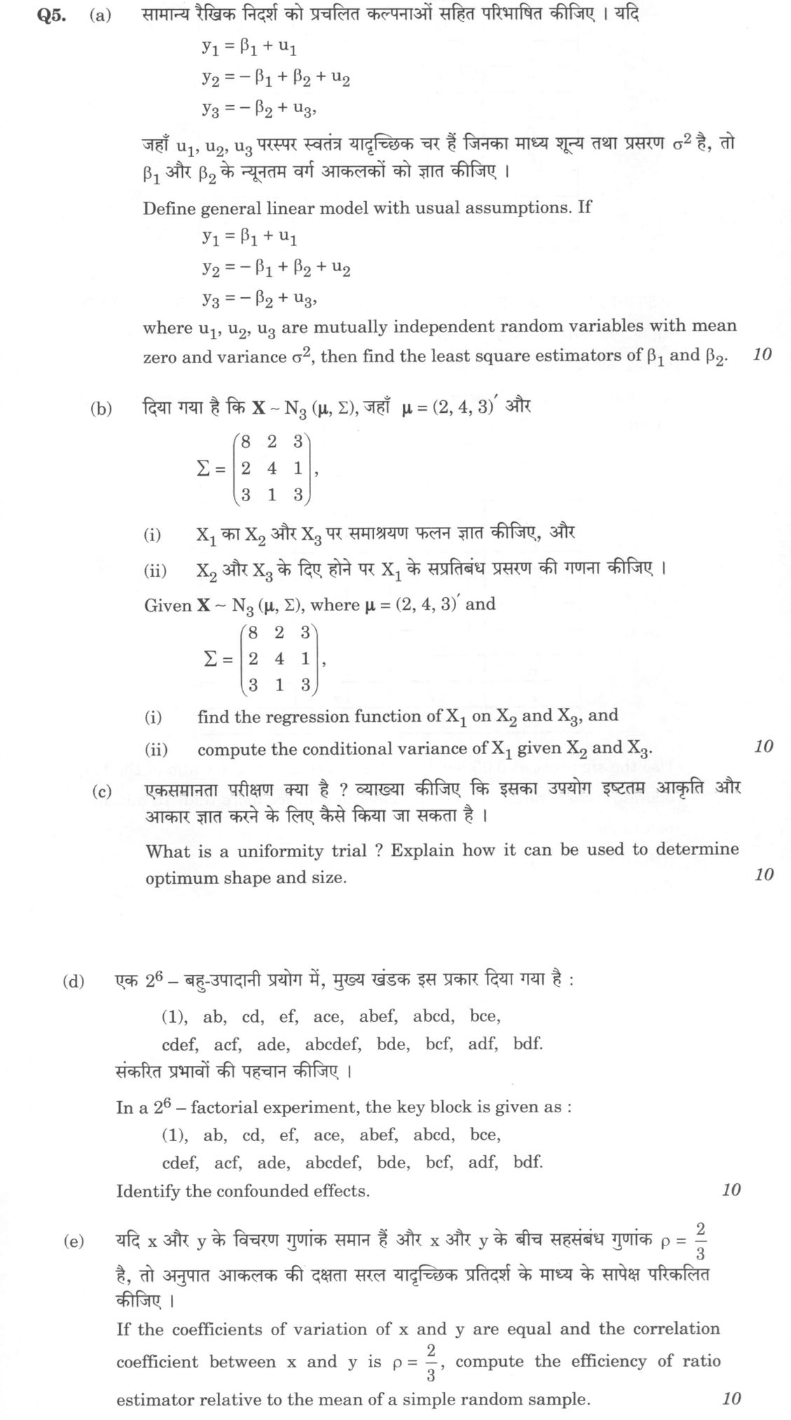
(a) Define general linear model with usual assumptions. If y₁ = β₁ + u₁, y₂ = –β₁ + β₂ + u₂, y₃ = –β₂ + u₃, where u₁, u₂, u₃ are…

(a) The general linear model is y = Xβ + u, where y is an n × 1 vector, X is a known n × p matrix of rank p, β is a p × 1 vector of unknown parameters, and u is the error vector. The usual assumptions are E(u) = 0, Var(u) = σ² Iₙ, and the components uᵢ are mutually independent; for distributional inference they are often taken to be normal, uᵢ ~ N(0, σ²). Here σ² has square units of y. The least squares estimator minimizes S(β) = (y - Xβ)'(y - Xβ). Differentiating with respect to β and setting the derivative to zero gives the normal equations X'Xβhat = X'y. The condition of validity is that X'X be nonsingular; this holds when X has full column rank. Hence βhat = (X'X)⁻¹X'y.

For the given model, y = (y₁, y₂, y₃)' and X = [ [1, 0], [-1, 1], [0, -1] ]. Then X'X = [ [2, -1], [-1, 2] ], whose determinant is 3, so (X'X)⁻¹ = (1/3)[ [2, 1], [1, 2] ], and X'y = (y₁ - y₂, y₂ - y₃)'. Hence β₁hat = (1/3)[2(y₁ - y₂) + (y₂ - y₃)] = (2y₁ - y₂ - y₃)/3, β₂hat = (1/3)[(y₁ - y₂) + 2(y₂ - y₃)] = (y₁ + y₂ - 2y₃)/3. Substituting these back gives fitted values yhat₁ = β₁hat, yhat₂ = -β₁hat + β₂hat, and yhat₃ = -β₂hat, and the residuals are orthogonal to the columns of X. β₁hat = (2y₁ - y₂ - y₃)/3, β₂hat = (y₁ + y₂ - 2y₃)/3.

(b) For X ~ N₃(μ, Σ) with positive definite covariance matrix, the conditional distribution of X₁ given X₂₃ = (X₂, X₃)' is normal. Partition μ = (μ₁, μ₂₃)' and Σ = [ [Σ₁₁, Σ₁₂₃], [Σ₁₂₃', Σ₂₃] ]. The conditional mean and variance are E(X₁ | X₂₃) = μ₁ + Σ₁₂₃ Σ₂₃⁻¹ (X₂₃ - μ₂₃), Var(X₁ | X₂₃) = Σ₁₁ - Σ₁₂₃ Σ₂₃⁻¹ Σ₁₂₃'. The formula requires Σ₂₃ to be nonsingular. Here μ₁ = 2, μ₂₃ = (4, 3)', Σ₁₁ = 8, Σ₁₂₃ = (2, 3), and Σ₂₃ = [ [4, 1], [1, 3] ]. The determinant of Σ₂₃ is 4 × 3 - 1 × 1 = 11, so Σ₂₃⁻¹ = (1/11)[ [3, -1], [-1, 4] ].

(i) Thus Σ₁₂₃ Σ₂₃⁻¹ = (2, 3)(1/11)[ [3, -1], [-1, 4] ] = (1/11)(2 × 3 + 3 × (-1), 2 × (-1) + 3 × 4) = (3/11, 10/11). Therefore the regression function of X₁ on X₂ and X₃ is E(X₁ | X₂, X₃) = 2 + (3/11)(X₂ - 4) + (10/11)(X₃ - 3) = (3X₂ + 10X₃ - 20)/11. Regression function: E(X₁ | X₂, X₃) = (3X₂ + 10X₃ - 20)/11.

(ii) For the conditional variance, (2, 3)Σ₂₃⁻¹(2, 3)' = (1/11)(2, 3)[ [3, -1], [-1, 4] ](2, 3)' = (1/11)(2, 3)(3, 10)' = (6 + 30)/11 = 36/11. Hence Var(X₁ | X₂, X₃) = 8 - 36/11 = (88 - 36)/11 = 52/11. As a check, this is less than the marginal variance 8, as required for a conditional variance. Conditional variance: 52/11, in square units of X₁.

(c) A uniformity trial is a preliminary field experiment in which a single uniform treatment, or no treatment, is applied to a large number of small plots in the field. The yields of these plots are measured to estimate the natural spatial variability of the field before the main experiment is laid out. It does not estimate treatment effects; it estimates field heterogeneity and is used to choose the shape and size of experimental plots. The trial should be conducted over the same field and under the same conditions as the main experiment, and the unit plots should be small enough to represent the smallest practical plot size.

• The field is first divided into convenient unit plots. Adjacent unit plots are then combined to form candidate plots of different sizes and shapes, for example 1 × 1, 2 × 1, 1 × 2, 2 × 2, and larger rectangles.
• For each candidate shape and size, the variance of the plot yields is computed. If two shapes have the same area, the shape with the smaller variance is preferred, because it gives smaller experimental error for the same land area.
• For a fixed shape, let Vₚ be the variance of a plot made up of p unit plots and V₁ the variance of one unit plot. Fairfield Smith's law is Vₚ = V₁ / pᵇ. The exponent b is estimated from the slope of log Vₚ against log p. b = 1 corresponds to independent unit-plot errors, i.e. no spatial correlation, often interpreted as a homogeneous field, so the variance of a p-unit plot is V₁/p. b = 0 corresponds to maximum spatial heterogeneity, so increasing plot size gives almost no reduction in variance. A larger b therefore indicates less heterogeneity and a greater gain from larger plots.
• The optimum size is chosen by balancing the reduction in Vₚ against the loss of degrees of freedom, the increase in cost, and the reduction in the number of plots when total area is fixed. In practice one chooses the size at which a cost- and degrees-of-freedom-adjusted measure of error variance stops giving a worthwhile reduction. If b is high, larger plots may be justified; if b is low, smaller plots are usually better.

(d) The key block has 16 treatments out of 64 in a 2⁶ factorial, so there are 4 blocks. Hence two independent effects are confounded with blocks, and their product is also confounded, giving three confounded effects. Represent each treatment by a binary vector (a, b, c, d, e, f), where a letter present is 1 and absent is 0. An effect is confounded if its sign is constant in the key block. Take the sign to be + when the number of letters of the effect present in a treatment is even, and - when it is odd. Since (1) is in the key block, a confounded effect with coefficient vector u = (u(a), u(b), u(c), u(d), u(e), u(f)) must satisfy u · x = 0 for every treatment x in the block, with all equalities modulo 2.

From the treatments ab, cd, and ef we get u(a) = u(b), u(c) = u(d), u(e) = u(f). From ace we get u(a) + u(c) + u(e) = 0. Thus the two independent solutions are u = (1, 1, 0, 0, 1, 1) and u = (0, 0, 1, 1, 1, 1), and their sum modulo 2 is u = (1, 1, 1, 1, 0, 0). These correspond to the effects abef, cdef, and abcd. In the given key block, every treatment contains an even number of letters from abcd, from abef, and from cdef, so the signs are constant. The other three blocks are obtained by multiplying the key block by any treatment not in it; the same three effects are constant in each block. Confounded effects: abcd, abef, cdef.

(e) Let Sx and Sy be the population standard deviations of x and y, and let Xbar and Ybar be the population means. For a simple random sample of size n with sampling fraction f, the variance of the sample mean is V(ybar) = (1 - f)Sy² / n. The ratio estimator of Ybar has approximate first-order variance V(ybar_r) = (1 - f)/n [Sy² + R²Sx² - 2RρSxSy], where R = Ybar / Xbar and ρ is the correlation between x and y. The finite population correction cancels in the ratio of the two variances.

Equal coefficients of variation mean Sx / Xbar = Sy / Ybar, so R = Ybar / Xbar = Sy / Sx. Substituting this in the ratio-estimator variance gives V(ybar_r) = (1 - f)Sy²/n [1 + 1 - 2ρ] = (1 - f)Sy²/n · 2(1 - ρ). For ρ = 2/3, V(ybar_r) = (1 - f)Sy²/n · 2/3. Taking efficiency relative to the sample mean as V(ybar) / V(ybar_r), the efficiency is 1 / (2/3) = 3/2 = 1.5, i.e. 150%. Equivalently, the ratio estimator has two-thirds of the variance of the sample mean. This shows that the ratio estimator is more efficient than the simple sample mean because the correlation is greater than 1/2. Efficiency = 3/2, or 150%; relative variance = 2/3.