Paper II — Q2
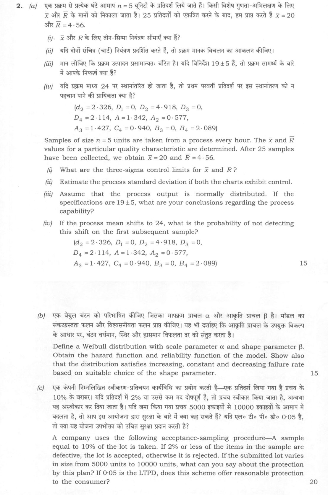
(a) Samples of size n = 5 units are taken from a process every hour. The x̄ and R̄ values for a particular quality characteristic…
Samples of size n = 5 units are taken from a process every hour. The x̄ and R̄ values for a particular quality characteristic are determined. After 25 samples have been collected, we obtain x̄̄ = 20 and R̄ = 4·56.
What are the three-sigma control limits for x̄ and R?
Estimate the process standard deviation if both the charts exhibit control.
Assume that the process output is normally distributed. If the specifications are 19 ± 5, what are your conclusions regarding the process capability?
If the process mean shifts to 24, what is the probability of not detecting this shift on the first subsequent sample?
(d₂ = 2·326, D₁ = 0, D₂ = 4·918, D₃ = 0, D₄ = 2·114, A = 1·342, A₂ = 0·577, A₃ = 1·427, C₄ = 0·940, B₃ = 0, B₄ = 2·089) 15 marks
Define a Weibull distribution with scale parameter α and shape parameter β. Obtain the hazard function and reliability function of the model. Show also that the distribution satisfies increasing, constant and decreasing failure rate based on suitable choice of the shape parameter. 15 marks
A company uses the following acceptance-sampling procedure—A sample equal to 10% of the lot is taken. If 2% or less of the items in the sample are defective, the lot is accepted, otherwise it is rejected. If the submitted lot varies in size from 5000 units to 10000 units, what can you say about the protection by this plan? If 0·05 is the LTPD, does this scheme offer reasonable protection to the consumer? 20 marks
हिंदी में प्रश्न पढ़ें
एक प्रक्रम से प्रत्येक घंटे आमाप n = 5 यूनिटों के प्रतिदर्श लिये जाते हैं। किसी विशेष गुणता-अभिलक्षण के लिए x̄ और R̄ के मानों को निकाला जाता है। 25 प्रतिदर्शों को एकत्रित करने के बाद, हम प्राप्त करते हैं x̄̄ = 20 और R̄ = 4·56।
x̄ और R के लिए तीन-सिग्मा नियंत्रण सीमाएँ क्या हैं?
यदि दोनों संचित्र (चार्ट) नियंत्रण प्रदर्शित करते हैं, तो प्रक्रम मानक विचलन का आकलन कीजिए।
मान लीजिए कि प्रक्रम उत्पादन प्रसामान्यतः बंटित है। यदि विनिर्देश 19 ± 5 हैं, तो प्रक्रम सामर्थ्य के बारे में आपके निष्कर्ष क्या हैं?
यदि प्रक्रम माध्य 24 पर स्थानांतरित हो जाता है, तो प्रथम परवर्ती प्रतिदर्श पर इस स्थानांतरण को न पहचान पाने की प्रायिकता क्या है?
(d₂ = 2·326, D₁ = 0, D₂ = 4·918, D₃ = 0, D₄ = 2·114, A = 1·342, A₂ = 0·577, A₃ = 1·427, C₄ = 0·940, B₃ = 0, B₄ = 2·089) 15 अंक
एक वेबुल बंटन को परिभाषित कीजिए जिसका मापक्रम प्राचल α और आकृति प्राचल β है। मॉडल का संकटप्रसूता फलन और विश्वसनीयता फलन प्राप्त कीजिए। यह भी दर्शाइए कि आकृति प्राचल के उपयुक्त विकल्प के आधार पर, बंटन वर्धमान, स्थिर और ह्रासमान विफलता दर को संतुष्ट करता है। 15 अंक
एक कंपनी निम्नलिखित स्वीकरण-प्रतिचयन कार्यविधि का प्रयोग करती है—एक प्रतिदर्श लिया गया है प्रचय के 10% के बराबर। यदि प्रतिदर्श में 2% या उससे कम मद दोषपूर्ण है, तो प्रचय स्वीकार किया जाता है, अन्यथा यह अस्वीकार कर दिया जाता है। यदि जमा किया गया प्रचय 5000 इकाइयों से 10000 इकाइयों के आमाप में बदलता है, तो आप इस आयोजना द्वारा सुरक्षा के बारे में क्या कह सकते हैं? यदि एल० टी० पी० डी० 0·05 है, तो क्या यह योजना उपभोक्ता को उचित सुरक्षा प्रदान करती है? 20 अंक
Model answer
Written by UPSC Answer Check against this question's marking rubric, to the expected length. UPSC does not publish answers for Mains — this is one way to score well, not an official key.
(a)(i) For the x̄ chart, A₂ = 0·577. CL = x̄̄ = 20. UCL = 20 + 0·577 × 4·56 = 20 + 2·63112 = 22·63112. LCL = 20 − 2·63112 = 17·36888. For the R chart, D₃ = 0, D₄ = 2·114. CL = 4·56, UCL = 2·114 × 4·56 = 9·63984, LCL = 0 × 4·56 = 0. Thus the three-sigma limits are:
- x̄ chart: (17·3689, 22·6311)
- R chart: (0, 9·6398)
(a)(ii) Since the charts exhibit control, estimate σ by σ = R̄/d₂, where d₂ = 2·326. σ = 4·56/2·326 = 1·96045. So the process standard deviation is approximately 1·960 units.
(a)(iii) Specifications are 19 ± 5, so LSL = 14, USL = 24, target = 19. Process mean ≈ 20, σ ≈ 1·96045. Cp = (USL − LSL)/(6σ) = 10/(6 × 1·96045) = 0·8501. Cpk = min((24 − 20)/(3σ), (20 − 14)/(3σ)) = min(4/5·8813, 6/5·8813) = min(0·6801, 1·0202) = 0·6801. The proportion nonconforming is P(X < 14) + P(X > 24) = Φ((14 − 20)/1·96045) + 1 − Φ((24 − 20)/1·96045) = Φ(−3·0605) + 1 − Φ(2·0404) ≈ 0·0011 + 0·0207 = 0·0218. Thus about 2·18% of output lies outside specifications. Since Cp < 1 and Cpk < 1, the process is not capable, and it is off-centre toward the upper specification.
(a)(iv) After the mean shifts to 24, x̄ has mean 24 and standard error σ_x̄ = σ/√n = 1·96045/√5 = 0·87674. Not detecting means x̄ remains between the x̄ control limits 17·36888 and 22·63112. β = P(17·36888 ≤ x̄ ≤ 22·63112 | μ = 24) = Φ((22·63112 − 24)/0·87674) − Φ((17·36888 − 24)/0·87674) = Φ(−1·5613) − Φ(−7·56) ≈ 0·0592 − 0 ≈ 0·0592. So the probability of not detecting the shift on the first subsequent sample is about 0·059, or 5·9%. The R chart is unaffected by a mean shift.
(b) A Weibull distribution with scale parameter α and shape parameter β has pdf f(x) = (β/α)(x/α)^(β−1) exp[−(x/α)^β], x > 0, α > 0, β > 0. Its CDF is F(x) = 1 − exp[−(x/α)^β]. Hence the reliability function is R(x) = 1 − F(x) = exp[−(x/α)^β]. The hazard function is h(x) = f(x)/R(x) = (β/α)(x/α)^(β−1) = (β/α^β)x^(β−1). Differentiate: h′(x) = (β/α^β)(β − 1)x^(β−2). Since β > 0 and x > 0, the sign of h′(x) is the sign of β − 1.
- If 0 < β < 1, then h′(x) < 0: decreasing failure rate.
- If β = 1, then h′(x) = 0 and h(x) = 1/α: constant failure rate.
- If β > 1, then h′(x) > 0: increasing failure rate. Thus the Weibull family can represent decreasing, constant and increasing failure rates depending on β.
(c) Let lot size be N, sample n = 0·10N, and acceptance number c = 0·02n = 0·002N. The exact distribution of the number defective D is hypergeometric: Pa(p) = sum over d = 0 to c of [C(K,d) C(N−K, n−d)] / C(N,n), where K = pN. For N = 5000: n = 500, c = 10. For N = 10000: n = 1000, c = 20.
Using the normal approximation to the hypergeometric with continuity correction: μ = np, Var = np(1−p)(N−n)/(N−1), Pa ≈ Φ((c + 0·5 − μ)/√Var).
At LTPD p = 0·05: For N = 5000: μ = 25, Var = 500 × 0·05 × 0·95 × (4500/4999) = 21·3793, sd = 4·6238. Pa ≈ Φ((10·5 − 25)/4·6238) = Φ(−3·136) ≈ 0·00086. For N = 10000: μ = 50, Var = 1000 × 0·05 × 0·95 × (9000/9999) = 42·7543, sd = 6·5387. Pa ≈ Φ((20·5 − 50)/6·5387) = Φ(−4·512) ≈ 3·2 × 10^−6. Both probabilities are far below 0·10, the usual consumer’s risk limit at LTPD. Hence the scheme offers very strong, indeed stricter than usual, protection to the consumer at LTPD = 0·05.
For comparison, at p = 0·02: For N = 5000: μ = 10, sd = 2·970, Pa ≈ Φ((10·5 − 10)/2·970) = Φ(0·168) ≈ 0·567. For N = 10000: μ = 20, sd = 4·200, Pa ≈ Φ((20·5 − 20)/4·200) = Φ(0·119) ≈ 0·547. Thus even lots with 2% defective have only about 55–57% acceptance, so producer’s risk is high. As lot size increases from 5000 to 10000, the sample size increases, the OC curve becomes steeper, and consumer protection improves further.
What "Solve" is asking you to do
Choose the method, then carry it through to a final answer. Identifying what kind of problem this is and why that method applies is the first thing marked; a correct figure arrived at invisibly earns almost nothing.
Structure that answers it
Given data and what is required → method chosen, with the reason it applies → set-up (equation, circuit, free body, trial balance) → working, step by step → answer with units and any condition of validity
Where marks are lost
Doing the middle steps mentally and writing only the result. In mathematics papers, a further loss comes from giving a decimal where the exact value in surds or fractions was wanted, or from skipping the justification a part explicitly asks for.
How this answer will be evaluated
Approach
(a) calculate: given > formula > substitution > result with units > interpretation | (b) derive: given > assumptions > stepwise derivation > result > check | (c) evaluate: criteria > evidence > balanced judgment Full marks: Complete derivations with clear interpretation and correct application of all constants and formulas.
Key points expected
- Calculate UCL/LCL for x-bar and R charts
- Estimate process standard deviation using d2
- Evaluate process capability against 19 ± 5 specs
- Compute probability of not detecting shift to 24
- Define Weibull PDF with scale and shape parameters
- Derive hazard function from PDF and CDF
- Derive reliability function from CDF
- Show IFR, CFR, DFR for beta > 1, = 1, < 1
Evaluation rubric
Each sub-part is marked on its own, against the marks and word limit printed on the paper.
- (a) Compute control limits, sigma, capability, and probability of non-detection. 15 marks
calculate— given → formula → substitution → result with units → interpretation
Must cover
- Calculate UCL/LCL for x-bar and R charts
- Estimate process standard deviation using d2
- Evaluate process capability against 19 ± 5 specs
- Compute probability of not detecting shift to 24
Loses marks
- Computation without interpretation of results
- Unstated assumptions regarding distribution
- Incorrect substitution of constants
Earns more
- Correct use of A2, D3, D4 constants
- Explicit statement of normality assumption
- Interpretation of capability index in context
- Correct application of z-score for probability
Extra mark
- Clean tabulation of constants used
- Explicit distinction between estimator and parameter
- (b) Define Weibull distribution and derive hazard and reliability functions. 15 marks
derive— given → assumptions → stepwise derivation → result → check
Must cover
- Define Weibull PDF with scale and shape parameters
- Derive hazard function from PDF and CDF
- Derive reliability function from CDF
- Show IFR, CFR, DFR for beta > 1, = 1, < 1
Loses marks
- Skipping derivation steps in hazard function
- Incorrect relationship between beta and failure rate
- Confusing scale and shape parameter roles
Earns more
- Correct notation for scale and shape parameters
- Stepwise derivation showing intermediate steps
- Clear explanation of failure rate behavior
- Consistent use of mathematical symbols
Extra mark
- Graphical representation of hazard function
- Physical interpretation of shape parameter
- (c) Evaluate acceptance sampling plan protection for varying lot sizes. 20 marks
evaluate— criteria → evidence → balanced judgment
Must cover
- Analyze protection for 5000 and 10000 unit lots
- Calculate sample sizes for both lot sizes
- Assess LTPD of 0.05 for consumer protection
- Compare protection levels across lot sizes
Loses marks
- Ignoring lot size variation in analysis
- No assessment of LTPD adequacy
- Computation without consumer protection judgment
Earns more
- Clear calculation of acceptance numbers
- Explicit discussion of producer and consumer risk
- Balanced judgment on plan adequacy
- Correct application of sampling theory
Extra mark
- OC curve sketch for the plan
- Reference to standard sampling tables
Practice this exact question
Write your answer and it is marked point by point against the model answer above — what you covered, what you missed, what you got wrong.
Evaluate my answer →More from Statistics 2022 Paper II
- Q1 (a) Distinguish between process control and product control. Explain the various sources…
- Q2 (a) Samples of size n = 5 units are taken from a process every hour. The x̄ and R̄ values…
- Q3 (a) It is planned to raise a research team to a strength of 50 chemists, which is to be m…
- Q4 (a) Use penalty method to solve the following linear programming problem : Maximize Z = x…
- Q5 (a) Apply the method of link relatives to the following data and calculate the seasonal i…