Paper I — Q5
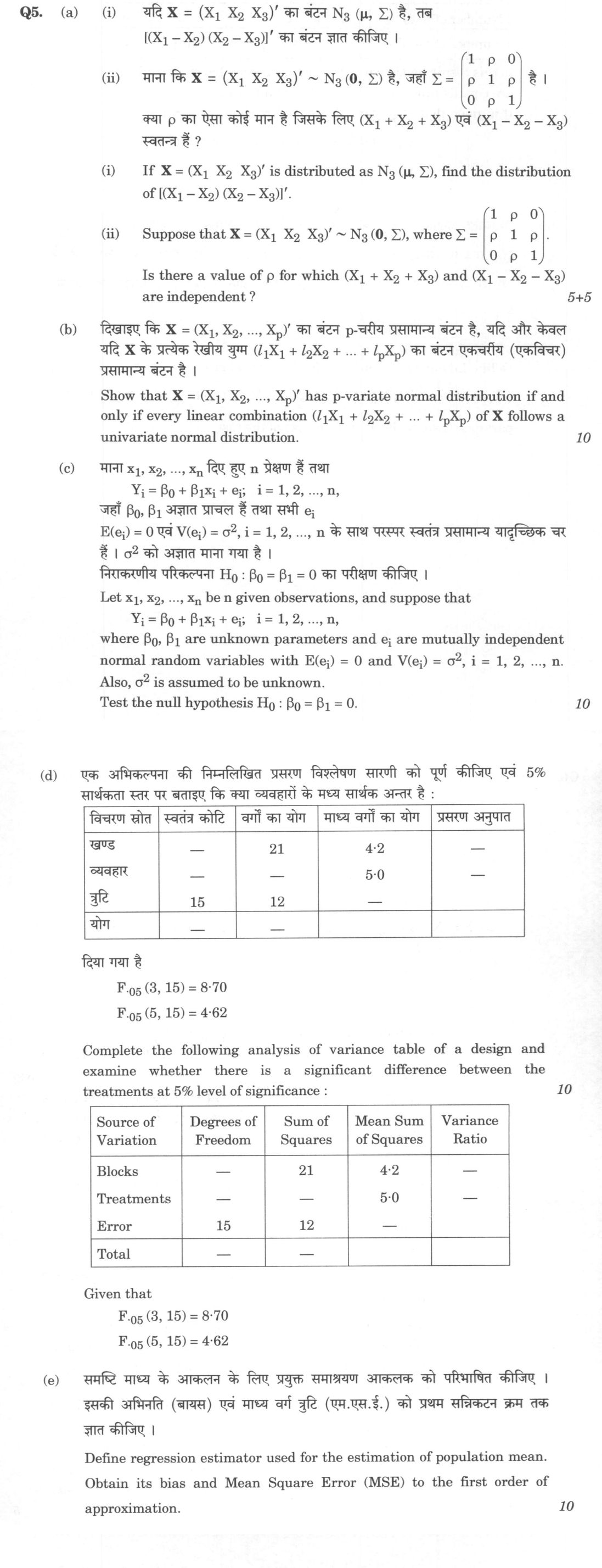
(a) (i) If **X** = (X₁ X₂ X₃)' is distributed as N₃ (μ, Σ), find the distribution of [(X₁ – X₂) (X₂ – X₃)]'. (5 marks) (ii)…
If **X** = (X₁ X₂ X₃)' is distributed as N₃ (μ, Σ), find the distribution of [(X₁ – X₂) (X₂ – X₃)]'. 5 marks
Suppose that **X** = (X₁ X₂ X₃)' ~ N₃ (**0**, Σ), where Σ = 1 & ρ & 0 ρ & 1 & ρ 0 & ρ & 1 . Is there a value of ρ for which (X₁ + X₂ + X₃) and (X₁ – X₂ – X₃) are independent ? 5 marks
Show that **X** = (X₁, X₂, ..., Xₚ)' has p-variate normal distribution if and only if every linear combination (l₁X₁ + l₂X₂ + ... + lₚXₚ) of **X** follows a univariate normal distribution. 10 marks
Let x₁, x₂, ..., xₙ be n given observations, and suppose that Yᵢ = β₀ + β₁xᵢ + eᵢ; i = 1, 2, ..., n, where β₀, β₁ are unknown parameters and eᵢ are mutually independent normal random variables with E(eᵢ) = 0 and V(eᵢ) = σ², i = 1, 2, ..., n. Also, σ² is assumed to be unknown. Test the null hypothesis H₀ : β₀ = β₁ = 0. 10 marks
Complete the following analysis of variance table of a design and examine whether there is a significant difference between the treatments at 5% level of significance:
| Source of Variation | Degrees of Freedom | Sum of Squares | Mean Sum of Squares | Variance Ratio |
|---|---|---|---|---|
| Blocks | — | 21 | 4·2 | — |
| Treatments | — | — | 5·0 | — |
| Error | 15 | 12 | — | |
| Total | — | — |
Given that F_·05(3, 15) = 8·70, F_·05(5, 15) = 4·62 10 marks
Define regression estimator used for the estimation of population mean. Obtain its bias and Mean Square Error (MSE) to the first order of approximation. 10 marks
हिंदी में प्रश्न पढ़ें
यदि **X** = (X₁ X₂ X₃)' का बंटन N₃ (μ, Σ) है, तब [(X₁ – X₂) (X₂ – X₃)]' का बंटन ज्ञात कीजिए । (5 अंक)
माना कि **X** = (X₁ X₂ X₃)' ~ N₃ (**0**, Σ) है, जहाँ Σ = 1 & ρ & 0 ρ & 1 & ρ 0 & ρ & 1 है । क्या ρ का ऐसा कोई मान है जिसके लिए (X₁ + X₂ + X₃) एवं (X₁ – X₂ – X₃) स्वतंत्र हैं ? (5 अंक)
दिखाइए कि **X** = (X₁, X₂, ..., Xₚ)' का बंटन p-चरिय प्रसामान्य बंटन है, यदि और केवल यदि **X** के प्रत्येक रैखीय युग्म (l₁X₁ + l₂X₂ + ... + lₚXₚ) का बंटन एकचरिय (एकविचर) प्रसामान्य बंटन है । (10 अंक)
माना x₁, x₂, ..., xₙ दिए हुए n प्रेक्षण हैं तथा Yᵢ = β₀ + β₁xᵢ + eᵢ; i = 1, 2, ..., n, जहाँ β₀, β₁ अज्ञात प्राचल हैं तथा सभी eᵢ E(eᵢ) = 0 एवं V(eᵢ) = σ², i = 1, 2, ..., n के साथ परस्पर स्वतंत्र प्रसामान्य यादृच्छिक चर हैं । σ² को अज्ञात माना गया है । निराकरणीय परिकल्पना H₀ : β₀ = β₁ = 0 का परीक्षण कीजिए । (10 अंक)
एक अभिकल्पना की निम्नलिखित प्रसरण विल्लेखन सारणी को पूर्ण कीजिए एवं 5% सार्थकता स्तर पर बताइए कि क्या व्यवहारों के मध्य सार्थक अंतर है :
| विचरण स्रोत | स्वतंत्र कोटि | वर्गों का योग | माध्य वर्गों का योग | प्रसरण अनुपात |
|---|---|---|---|---|
| खंड | — | 21 | 4·2 | — |
| व्यवहार | — | — | 5·0 | — |
| त्रुटि | 15 | 12 | — | |
| योग | — | — |
दिया गया है F_·05(3, 15) = 8·70, F_·05(5, 15) = 4·62 (10 अंक)
समष्टि माध्य के आकलन के लिए प्रयुक्त समाश्रयण आकलक को परिभाषित कीजिए । इसकी अभिनति (बायस) एवं माध्य वर्ग त्रुटि (एम.एस.ई.) को प्रथम सन्निकटन क्रम तक प्राप्त कीजिए । (10 अंक)
Model answer
Written by UPSC Answer Check against this question's marking rubric, to the expected length. UPSC does not publish answers for Mains — this is one way to score well, not an official key.
(a)(i) Let Y = [(X₁ − X₂), (X₂ − X₃)]′. Then Y = AX, where A = [[1, −1, 0], [0, 1, −1]]. Since X ∼ N₃(μ, Σ), by the linear-transformation theorem for multivariate normal vectors, Y ∼ N₂(Aμ, AΣA′).
Here Aμ = [μ₁ − μ₂, μ₂ − μ₃]′. Also, if Σ = (σᵢⱼ), then Var(X₁ − X₂) = σ₁₁ + σ₂₂ − 2σ₁₂, Var(X₂ − X₃) = σ₂₂ + σ₃₃ − 2σ₂₃, Cov(X₁ − X₂, X₂ − X₃) = σ₁₂ − σ₁₃ − σ₂₂ + σ₂₃.
Hence Y ∼ N₂([μ₁ − μ₂, μ₂ − μ₃]′, [[σ₁₁ + σ₂₂ − 2σ₁₂, σ₁₂ − σ₁₃ − σ₂₂ + σ₂₃], [σ₁₂ − σ₁₃ − σ₂₂ + σ₂₃, σ₂₂ + σ₃₃ − 2σ₂₃]]).
(a)(ii) Let U = X₁ + X₂ + X₃, V = X₁ − X₂ − X₃. Since U and V are linear combinations of a multivariate normal vector, (U, V) is jointly normal. Therefore U and V are independent if and only if Cov(U, V) = 0.
Using Σ = [[1, ρ, 0], [ρ, 1, ρ], [0, ρ, 1]], Cov(U, V) = (1, 1, 1) Σ (1, −1, −1)′. Compute: = 1 − ρ + ρ − 1 − ρ − ρ − 1 = −1 − 2ρ.
Set this equal to zero: −1 − 2ρ = 0 ⇒ ρ = −1/2.
For ρ = −1/2, Σ is positive definite because its leading minors are positive and det(Σ) = 1 − 2ρ² = 1 − 1/2 = 1/2 > 0. Yes, for ρ = −1/2, U and V are independent.
(b) Let X = (X₁, X₂, ..., Xₚ)′.
First suppose X ∼ Nₚ(μ, Σ). For any fixed vector l = (l₁, l₂, ..., lₚ)′, the linear combination L = l₁X₁ + l₂X₂ + ... + lₚXₚ = l′X is a linear transformation of X. By the linear-transformation property of multivariate normal distribution, L ∼ N(l′μ, l′Σl). If l′Σl = 0, L is a degenerate univariate normal random variable. Thus every linear combination is univariate normal.
Conversely, suppose every linear combination l′X is univariate normal. Define μ = (E X₁, E X₂, ..., E Xₚ)′, Σ = (Cov(Xᵢ, Xⱼ)). For any t = (t₁, ..., tₚ)′, the random variable t′X is normal. Its mean is E(t′X) = t′μ, and its variance is Var(t′X) = t′Σt. Therefore its characteristic function is E exp(i t′X) = exp(i t′μ − (1/2)t′Σt).
But this is exactly the characteristic function of Nₚ(μ, Σ). By uniqueness of characteristic functions, X ∼ Nₚ(μ, Σ). Hence X has a p-variate normal distribution if and only if every linear combination of its components is univariate normal.
(c) The model is Yᵢ = β₀ + β₁xᵢ + eᵢ, eᵢ ∼ N(0, σ²), independently, i = 1, ..., n. We test H₀ : β₀ = β₁ = 0 against H₁ : not both zero.
Let x̄ = (1/n)Σxᵢ, Ȳ = (1/n)ΣYᵢ, Sₓₓ = Σ(xᵢ − x̄)², Sₓᵧ = Σ(xᵢ − x̄)(Yᵢ − Ȳ), Sᵧᵧ = Σ(Yᵢ − Ȳ)².
Under the full model, the least-squares estimators are β̂₁ = Sₓᵧ / Sₓₓ, β̂₀ = Ȳ − β̂₁x̄. The full-model residual sum of squares is SSE_F = Σ(Yᵢ − β̂₀ − β̂₁xᵢ)² = Sᵧᵧ − Sₓᵧ² / Sₓₓ, with degrees of freedom n − 2.
Under H₀ : β₀ = β₁ = 0, the fitted value is 0, so SSE_R = ΣYᵢ² = Sᵧᵧ + nȲ². The number of restrictions is 2. Therefore the F statistic is F = [(SSE_R − SSE_F)/2] / [SSE_F/(n − 2)] = [(nȲ² + Sₓᵧ²/Sₓₓ)/2] / [(Sᵧᵧ − Sₓᵧ²/Sₓₓ)/(n − 2)].
Under H₀, F ∼ F₂,ₙ₋₂. Reject H₀ at level α if F > F_α;2,n−2. This requires n > 2 and Sₓₓ > 0.
(d) From the block row: MSS = SS/df ⇒ 4.2 = 21/df ⇒ df for blocks = 21/4.2 = 5.
Error MSS = 12/15 = 0.8.
Blocks df = 5 ⇒ number of blocks b = 6. Error df = (b − 1)(t − 1) = 15 ⇒ 5(t − 1) = 15 ⇒ t = 4. Thus treatments df = t − 1 = 3.
Treatments MSS = 5.0, so Treatments SS = 5.0 × 3 = 15.
Total df = 5 + 3 + 15 = 23. Total SS = 21 + 15 + 12 = 48.
Completed ANOVA entries:
- Blocks: df = 5, SS = 21, MSS = 4.2, VR = 4.2/0.8 = 5.25.
- Treatments: df = 3, SS = 15, MSS = 5.0, VR = 5.0/0.8 = 6.25.
- Error: df = 15, SS = 12, MSS = 0.8, VR = —.
- Total: df = 23, SS = 48, MSS = —, VR = —.
For treatments, the critical value is F₀.₀₅(3,15) = 8.70. Since observed F = 6.25 < 8.70, we fail to reject H₀. There is no significant difference between treatments at the 5% level. For completeness, blocks show F = 5.25 > F₀.₀₅(5,15) = 4.62, so blocks differ significantly.
(e) Let Y be the study variable and X an auxiliary variable whose population mean X̄ is known. In simple random sampling without replacement of size n, let ȳ and x̄ be sample means. The regression estimator of the population mean Ȳ is ȳ_lr = ȳ + b(X̄ − x̄), where b = sₓᵧ/sₓ² = Σ(xᵢ − x̄)(yᵢ − ȳ) / Σ(xᵢ − x̄)². If the population regression coefficient β is known, the estimator is ȳ_reg = ȳ + β(X̄ − x̄).
For the usual case where b is estimated, define population moments about means: μ₂₀ = (1/N)Σ(Xᵢ − X̄)², μ₀₂ = (1/N)Σ(Yᵢ − Ȳ)², μ₁₁ = (1/N)Σ(Xᵢ − X̄)(Yᵢ − Ȳ), μ₂₁ = (1/N)Σ(Xᵢ − X̄)²(Yᵢ − Ȳ), μ₃₀ = (1/N)Σ(Xᵢ − X̄)³, and β = μ₁₁/μ₂₀. Let f = n/N.
To the first order of approximation, the bias of ȳ_lr is B(ȳ_lr) = − (1 − f)/(n μ₂₀) (μ₂₁ − β μ₃₀) = (1 − f)/(n μ₂₀) (β μ₃₀ − μ₂₁).
Its mean square error to the first order is MSE(ȳ_lr) ≈ (1 − f)/n [μ₀₂ + β² μ₂₀ − 2β μ₁₁] = (1 − f)/n [μ₀₂ − μ₁₁²/μ₂₀] = (1 − f)/n S_Y²(1 − ρ²), where ρ = μ₁₁/√(μ₂₀ μ₀₂) is the population correlation coefficient between X and Y. The bias squared is of order n⁻² and is omitted. These results require large n, SRSWOR, μ₂₀ > 0, and known population mean X̄.
What "Solve" is asking you to do
Choose the method, then carry it through to a final answer. Identifying what kind of problem this is and why that method applies is the first thing marked; a correct figure arrived at invisibly earns almost nothing.
Structure that answers it
Given data and what is required → method chosen, with the reason it applies → set-up (equation, circuit, free body, trial balance) → working, step by step → answer with units and any condition of validity
Where marks are lost
Doing the middle steps mentally and writing only the result. In mathematics papers, a further loss comes from giving a decimal where the exact value in surds or fractions was wanted, or from skipping the justification a part explicitly asks for.
How this answer will be evaluated
Approach
Framework: Linear Model Theory and ANOVA. (a) calculate: given > formula > substitution > result with units > interpretation | (b) explain: definition/context > points in order > small example > short close | (c) calculate: given > formula > substitution > result with units > interpretation | (d) calculate: given > formula > substitution > result with units > interpretation | (e) explain: definition/context > points in order > small example > short close Full marks: Rigorous derivations, correct notation, complete tables, clear interpretations.
Key points expected
- Multivariate normal transformation properties
- Cramér-Wold theorem application
- F-test for joint hypothesis in regression
- ANOVA table completion and F-test
- Regression estimator bias and MSE derivation
Evaluation rubric
Each sub-part is marked on its own, against the marks and word limit printed on the paper.
- (a) Derive distribution of linear combination and check independence condition. 10 marks
calculate— given → formula → substitution → result with units → interpretation
Must cover
- Define transformation matrix A for (i)
- Compute mean vector Aμ
- Compute covariance matrix AΣA'
- Set covariance of linear forms to zero for (ii)
Loses marks
- Missing covariance calculation
- Assuming independence without proof
Earns more
- Explicitly state multivariate normal property
- Solve for ρ correctly
Extra mark
- Verify positive definiteness of Σ
- (b) Prove the Cramér-Wold theorem for multivariate normality. 10 marks
explain— definition/context → points in order → small example → short close
Must cover
- State characteristic function of X
- Show linear combination is univariate normal
- Use uniqueness of characteristic functions
- Conclude X is multivariate normal
Loses marks
- Proving only one direction
- Vague hand-waving on characteristic functions
Earns more
- Clear 'if and only if' structure
- Correct notation for l'X
Extra mark
- Mention Cramér-Wold theorem by name
- (c) Construct F-test for joint significance of regression coefficients. 10 marks
calculate— given → formula → substitution → result with units → interpretation
Must cover
- State H0 and H1 clearly
- Define F-statistic formula (R²/(1-R²) form)
- Identify degrees of freedom (2, n-3)
- State decision rule
Loses marks
- Using t-test for joint hypothesis
- Wrong degrees of freedom
Earns more
- Mention unknown σ² handled by F-test
- Correct notation for R²
Extra mark
- Alternative form using SSR/SSE
- (d) Complete ANOVA table and test treatment significance. 10 marks
calculate— given → formula → substitution → result with units → interpretation
Must cover
- Calculate missing degrees of freedom
- Calculate missing Sum of Squares
- Calculate F-ratio for treatments
- Compare with F-critical value
Loses marks
- Arithmetic errors in table
- Failing to compare with critical value
Earns more
- Clean, complete table
- Correct interpretation of F-test
Extra mark
- Explicit statement of null hypothesis
- (e) Define regression estimator and derive its bias and MSE. 10 marks
explain— definition/context → points in order → small example → short close
Must cover
- Define estimator formula (ȳ + b(x̄ - X̄))
- State first-order approximation assumption
- Derive bias term
- Derive MSE term
Loses marks
- Confusing estimator with parameter
- Missing first-order approximation step
Earns more
- Correct notation for population vs sample means
- Clear definition of b (regression coefficient)
Extra mark
- Mention condition for zero bias
Practice this exact question
Write your answer and it is marked point by point against the model answer above — what you covered, what you missed, what you got wrong.
Evaluate my answer →More from Statistics 2023 Paper I
- Q2 (a) Let X, Y, Z be three mutually independent standard exponential variates and W₁ = X +…
- Q3 (a) (i) If X is a random variable with finite variance, show that lim n² P{|X| > n} = 0.…
- Q4 (a) What is the role of properties of completeness and sufficiency in Statistical Inferen…
- Q5 (a) (i) If **X** = (X₁ X₂ X₃)' is distributed as N₃ (μ, Σ), find the distribution of [(X₁…
- Q6 (a) Let **X** = (X₁ X₂ X₃)' be distributed as N₃ (μ, Σ), where μ = (2 −1 3)' and Σ = 4 &…
- Q7 (a) Discuss the difference between sampling for variables and sampling for attributes wit…
- Q8 (a) Differentiate between randomised block design and balanced incomplete block design. I…