Paper II — Q1
(a) What do you understand by Statistical Quality Control (SQC)? Discuss briefly its need and utility in Industry. Discuss the…
What do you understand by Statistical Quality Control (SQC)? Discuss briefly its need and utility in Industry. Discuss the causes of variation in quality. 10 marks
Consider an item with failure rate Z(t) = t/(t+1). Write down the survivor function R(t) and hence evaluate Mean Time To Failure (MTTF). Also obtain the conditional survival function and Mean Residual Life (MRL). 10 marks
Solve the following linear programming problem by using graphical approach:
Minimize 4x₁ + 5x₂ + 6x₃
Subject to x₁ + x₂ ≥ 11 x₁ - x₂ ≤ 5 x₃ - x₁ - x₂ = 0 7x₁ + 12x₂ ≥ 35 x₁ ≥ 0, x₂ ≥ 0, x₃ ≥ 0 10 marks
In a two-person zero-sum game, write the payoff matrix in general notation. Consider the two-person zero-sum game where each player tosses an unbiased coin simultaneously. Player B pays ₹7 to A if H, H occurs or T, T occurs otherwise player A pays ₹3 to B. Write down A's payoff matrix. Explain the Max Min criterion for player A and hence define the saddle point. 10 marks
Let Xₜ be the state of a flea at time t
Find the transition Matrix P. Also obtain Pᵣ[X₂ = 3 | X₀ = 1]. 10 marks
हिंदी में प्रश्न पढ़ें
सांख्यिकी गुणवत्ता नियंत्रण (एस. क्यू. सी.) से आप क्या समझते हैं ? उद्योग में इसकी आवश्यकता एवं उपयोगिता पर संक्षेप में चर्चा कीजिए । गुणवत्ता में परिवर्तन के कारणों पर चर्चा कीजिए । (10 अंक)
विफलता दर Z(t) = t/(t+1) वाले किसी वस्तु (आइटम) पर विचार कीजिए । उत्तरजीविता फलन R(t) लिखिए और इस तरह विफलता तक माध्य काल (एम.टी.टी.एफ.) ज्ञात कीजिए । सप्रतिबन्ध उत्तरजीविता फलन एवं औसत अवशिष्ट जीवन (एम.आर.एल.) भी ज्ञात कीजिए । (10 अंक)
निम्नलिखित रैखिक प्रोग्रामन समस्या को ग्राफी विधि का उपयोग करके हल कीजिए :
न्यूनतमीकरण 4x₁ + 5x₂ + 6x₃
निम्न प्रतिबन्धों के अन्तर्गत x₁ + x₂ ≥ 11 x₁ - x₂ ≤ 5 x₃ - x₁ - x₂ = 0 7x₁ + 12x₂ ≥ 35 x₁ ≥ 0, x₂ ≥ 0, x₃ ≥ 0 (10 अंक)
द्वि-व्यक्ति शून्य-योगी खेल में, सामान्य संकेतन में भुगतान आव्यूह लिखिए । द्वि-व्यक्ति शून्य-योगी खेल पर विचार करें जहाँ प्रत्येक खिलाड़ी एक साथ ही एक निष्पक्ष सिक्का उछालता है । खिलाड़ी B, A को 7 रुपये का भुगतान करता है यदि H, H घटित होता है या T, T घटित होता है अन्यथा खिलाड़ी A, B को 3 रुपये का भुगतान करता है । A का भुगतान आव्यूह लिखिए । खिलाड़ी A के लिए अधिकतम-न्यूनतम (मैक्स मिन) निकष की व्याख्या कीजिए और इस तरह पल्यायन बिन्दु को परिभाषित कीजिए । (10 अंक)
मान लीजिए कि समय t पर Xₜ एक पिस्सू की अवस्था है।
संक्रमण आव्यूह P ज्ञात कीजिए। Pᵣ[X₂ = 3 | X₀ = 1] भी प्राप्त कीजिए। (10 अंक)
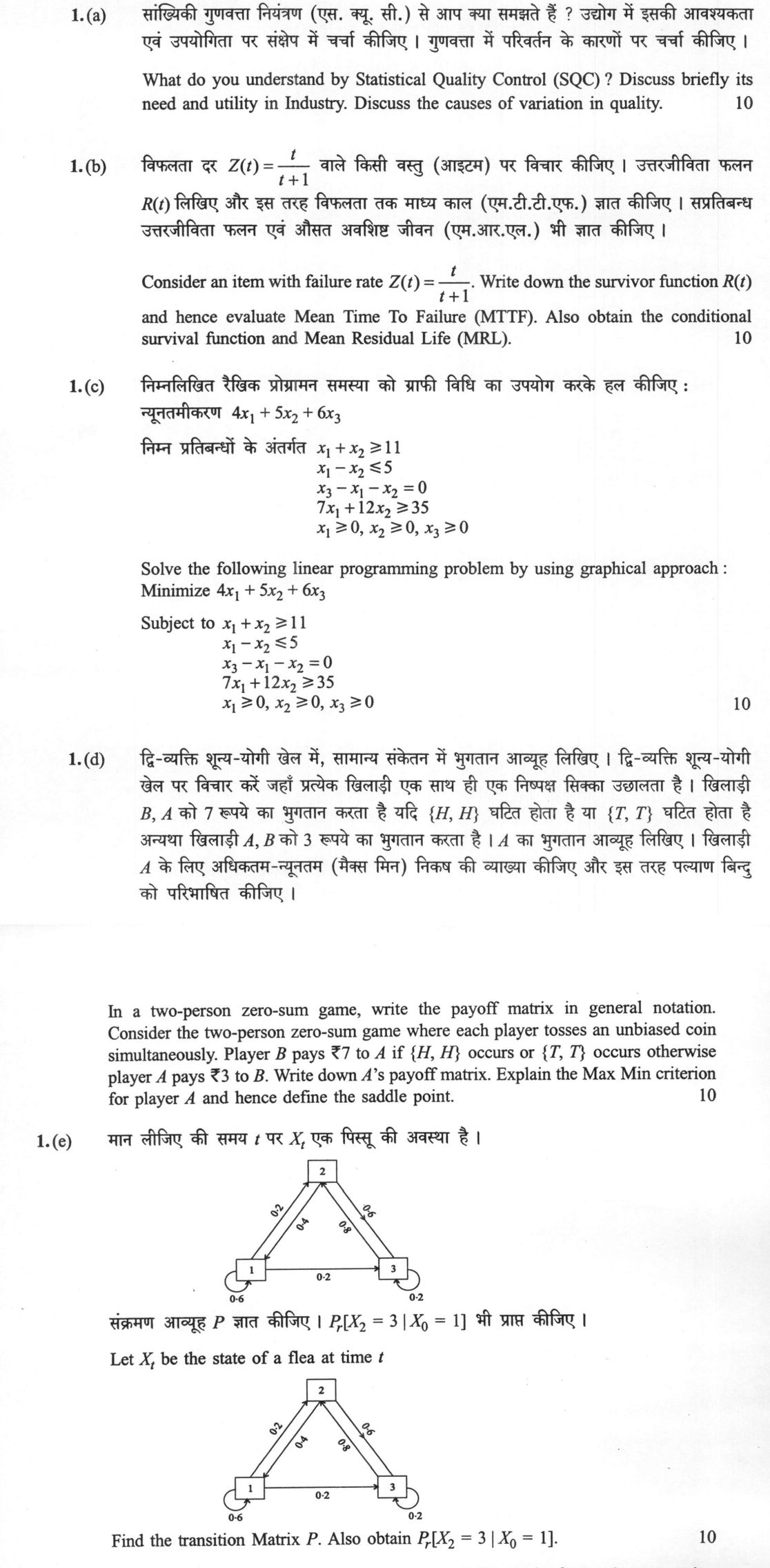
The figure this question refers to, in words
The question paper is a scan and the diagram did not survive as text. This is the figure as read from the original page — every component, value and label — so the question can be worked from the text below.
(e) A state transition diagram with three states represented by square boxes labeled 1, 2, and 3. State 2 is at the top, State 1 is at the bottom left, and State 3 is at the bottom right. Directed arrows indicate transitions with the following probabilities: From State 1 to State 2 (0.2), From State 1 to State 3 (0.2), From State 1 to State 1 (0.6, self-loop), From State 2 to State 1 (0.4), From State 2 to State 3 (0.6), From State 3 to State 2 (0.8), From State 3 to State 3 (0.2, self-loop).
Table: Cumulative Normal Distribution. Formula: phi(x) = integral from -infinity to x of (1/sqrt(2pi)) * e^(-t^2/2) dt. The table lists values of X in the first column (rows) and the second decimal place in the header row (columns). The body contains the corresponding cumulative probability values. Rows range from 0.0 to 3.4. Columns range from .00 to .09. Example values: X=0.0, col .00 is .5000; X=1.0, col .00 is .8413; X=2.0, col .00 is .9772. A bottom section lists specific x values (1.282, 1.645, 1.960, 2.326, 2.576, 3.090, 3.291, 3.891, 4.417) with their corresponding phi(x) values (e.g., 1.282 -> .90) and 2[1-phi(x)] values (e.g., 1.282 -> .20).
Model answer
Written by UPSC Answer Check against this question's marking rubric, to the expected length. UPSC does not publish answers for Mains — this is one way to score well, not an official key.
(a) Statistical Quality Control (SQC) is the use of statistical methods to monitor, control and improve the quality of products and processes. It treats quality as a measurable characteristic affected by random and assignable causes, and uses sampling inspection, acceptance sampling, control charts, process capability studies and design of experiments to decide whether a process is stable, capable and improving. SQC is not only final inspection; it is process control. It converts quality decisions from subjective judgment into evidence-based decisions, and it is especially useful when production is continuous, costly, or customer-sensitive. Control charts plot sample statistics such as mean, range or standard deviation against time and use upper and lower control limits. If points stay within limits and show no non-random pattern, the process is in statistical control. If a point exceeds a limit or a trend, cycle or run appears, a special cause is investigated. Its need in industry is to reduce defects, scrap, rework and warranty costs; to detect abnormal shifts before large batches are spoiled; to give objective evidence of process stability; to ensure consistent customer satisfaction; and to support continuous improvement and certification. Its utility is that it separates normal variation from abnormal variation, focuses management on process causes rather than only final inspection, and gives a common quantitative language for quality decisions. Causes of variation are of two types. Common-cause variation is inherent and random, arising from the system itself: small differences in material, machine wear, temperature, humidity, operator technique, measurement error and method. Special-cause or assignable-cause variation is due to identifiable disturbances: tool breakage, wrong material, power fluctuation, operator mistake, maintenance fault or a change in procedure. The 6M framework, Man, Machine, Material, Method, Measurement and Mother Nature, is often used to classify these sources. SQC aims to remove special causes and reduce common causes.
(b) Let T be the lifetime and Z(t)=t/(t+1) be the failure rate for t≥0. The formula is valid for t≥0 and assumes Z(t) is the hazard rate of a non-negative lifetime. By definition, Z(t) = -d/dt ln R(t), where R(t)=P(T>t). Hence ln R(t) = -∫ from 0 to t Z(u) du. Now ∫ from 0 to t u/(u+1) du = ∫ from 0 to t (1 - 1/(u+1)) du = [u - ln(u+1)] from 0 to t = t - ln(t+1). Therefore R(t) = exp[-t + ln(t+1)] = (t+1)exp(-t), t≥0. This satisfies R(0)=1 and R(t)→0. The density is f(t)=Z(t)R(t)=t exp(-t). MTTF = E[T] = ∫ from 0 to ∞ R(t) dt = ∫ from 0 to ∞ (t+1)exp(-t) dt = ∫ from 0 to ∞ t exp(-t) dt + ∫ from 0 to ∞ exp(-t) dt = 1 + 1 = 2 time units. For the conditional survivor function, let s≥0 be current age and t≥0 be additional time. R(t | s) = P(T > s+t | T > s) = R(s+t)/R(s) = [(t+s+1)exp(-(t+s))]/[(s+1)exp(-s)] = ((t+s+1)/(s+1))exp(-t). MRL at age s is m(s)=E[T-s | T>s] = ∫ from 0 to ∞ R(u | s) du = ∫ from 0 to ∞ [(u+s+1)/(s+1)]exp(-u) du = (1/(s+1))[∫ from 0 to ∞ u exp(-u) du + (s+1)∫ from 0 to ∞ exp(-u) du] = (1/(s+1))[1 + (s+1)] = (s+2)/(s+1) time units. At s=0, m(0)=2, agreeing with MTTF.
(c) The equality x₃ - x₁ - x₂ = 0 gives x₃ = x₁ + x₂. Since x₁, x₂ ≥ 0, x₃ ≥ 0 automatically. Substitute in the objective: 4x₁ + 5x₂ + 6x₃ = 4x₁ + 5x₂ + 6(x₁+x₂) = 10x₁ + 11x₂. The problem becomes minimize C = 10x₁ + 11x₂ subject to x₁ + x₂ ≥ 11, x₁ - x₂ ≤ 5, x₁ ≥ 0, x₂ ≥ 0. The graphical method is applicable because the equality constraint removes one variable, so the original three-dimensional feasible set is represented in the x₁-x₂ plane. The constraint 7x₁ + 12x₂ ≥ 35 is redundant because x₁ + x₂ ≥ 11 and x₂ ≥ 0 imply 7x₁ + 12x₂ = 7(x₁+x₂) + 5x₂ ≥ 77 > 35. Graphically, draw L₁: x₁ + x₂ = 11 with intercepts (11,0) and (0,11); the feasible side is above this line. Draw L₂: x₁ - x₂ = 5, or x₂ = x₁ - 5, with intercepts (5,0) and (0,-5); the feasible side is x₂ ≥ x₁ - 5, i.e. above this line in the x₁-x₂ plane. The intersection of L₁ and L₂ is found from x₁ + x₂ = 11 and x₁ - x₂ = 5, giving 2x₁ = 16, so x₁ = 8 and x₂ = 3. The feasible region is an unbounded convex polygonal region, with boundary segment from (0,11) to (8,3), a vertical ray x₁ = 0, x₂ ≥ 11, and a ray x₂ = x₁ - 5, x₁ ≥ 8. Because the objective is linear, if a finite minimum exists it must occur at an extreme point or along an edge; checking the extreme points and the directions of the unbounded edges is sufficient. Objective contours are 10x₁ + 11x₂ = C, straight lines of slope -10/11. Decreasing C moves the contour toward the origin; the first point of contact with the feasible region is the corner (8,3). Check corner values: at (0,11), C = 121; at (8,3), C = 113. Along the ray x₁ = 0, C = 11x₂, increasing for x₂ ≥ 11. Along the ray x₂ = x₁ - 5, C = 10x₁ + 11(x₁-5) = 21x₁ - 55, increasing for x₁ ≥ 8. Hence the minimum occurs at x₁ = 8, x₂ = 3, and x₃ = 8 + 3 = 11. The minimum value is 4(8) + 5(3) + 6(11) = 32 + 15 + 66 = 113 cost units.
(d) In a two-person zero-sum game, let player A have m pure strategies and player B have n pure strategies. The payoff matrix to A is written in general notation as A = (a(i,j)), i = 1,...,m, j = 1,...,n, where a(i,j) is the amount received by A when A chooses row i and B chooses column j. A maximizes payoff and B minimizes it. The payoff matrix is written from A's perspective; B's payoff would be the negative of this matrix. For the coin game, take A's rows as H and T, and B's columns as H and T. If HH or TT occurs, B pays ₹7 to A, so A's payoff is +7. If HT or TH occurs, A pays ₹3 to B, so A's payoff is -3. Thus A's payoff matrix is A = [7, -3; -3, 7]. The Max Min criterion for A is: for each row, find the minimum payoff, the worst outcome if B chooses optimally against that row, and then choose the row with the largest of these row minima. Row H has minimum min(7,-3) = -3. Row T has minimum min(-3,7) = -3. Therefore A's maximin value is max(-3,-3) = -3 ₹. For B, using the same A-payoff matrix, the minimax value is min(max(7,-3), max(-3,7)) = min(7,7) = 7 ₹. A saddle point is an entry a(i,j) that is simultaneously the minimum of its row and the maximum of its column; equivalently, the maximin value equals the minimax value, and that common value is the value of the game. If a saddle point existed, both players would have optimal pure strategies and no randomization would be needed. Here maximin -3 is not equal to minimax 7, so there is no saddle point in pure strategies.
(e) Let P(i,j) be the probability of moving from state i to state j in one step, with rows as current state and columns as next state. From the transition diagram, the one-step transition matrix is P = [3/5, 1/5, 1/5; 2/5, 0, 3/5; 0, 4/5, 1/5], i.e. [0.6, 0.2, 0.2; 0.4, 0.0, 0.6; 0.0, 0.8, 0.2]. The transition matrix is row-stochastic: each row sums to 1, so it is a valid Markov transition matrix. The calculation uses the Markov property and time-homogeneous transition probabilities, so the two-step probability is the (1,3) entry of P squared. The required probability is Pᵣ[X₂ = 3 | X₀ = 1] = (P²)(1,3). Compute the (1,3) entry of P²: (P²)(1,3) = (3/5)(1/5) + (1/5)(3/5) + (1/5)(1/5) = 3/25 + 3/25 + 1/25 = 7/25. This is also the sum of the two-step paths 1→1→3, 1→2→3, and 1→3→3.
What "Solve" is asking you to do
Choose the method, then carry it through to a final answer. Identifying what kind of problem this is and why that method applies is the first thing marked; a correct figure arrived at invisibly earns almost nothing.
Structure that answers it
Given data and what is required → method chosen, with the reason it applies → set-up (equation, circuit, free body, trial balance) → working, step by step → answer with units and any condition of validity
Where marks are lost
Doing the middle steps mentally and writing only the result. In mathematics papers, a further loss comes from giving a decimal where the exact value in surds or fractions was wanted, or from skipping the justification a part explicitly asks for.
How this answer will be evaluated
Approach
(a) discuss: intro > 3-4 dimensions > example > balanced close | (b) calculate: given > formula > substitution > result with units > interpretation | (c) calculate: given > formula > substitution > result with units > interpretation | (d) explain: definition/context > points in order > small example > short close | (e) calculate: given > formula > substitution > result with units > interpretation Full marks: All parts fully answered with correct derivations, clear diagrams, and proper interpretation.
Key points expected
- Define Statistical Quality Control (SQC)
- Explain need and utility in industry
- List causes of variation in quality
- Distinguish common vs special causes
- Derive survivor function R(t) from Z(t)
- Calculate Mean Time To Failure (MTTF)
- Obtain conditional survival function
- Calculate Mean Residual Life (MRL)
Evaluation rubric
Each sub-part is marked on its own, against the marks and word limit printed on the paper.
- (a) Definition of SQC, its industrial utility, and causes of quality variation. 10 marks
discuss— intro → 3-4 dimensions → example → balanced close
Must cover
- Define Statistical Quality Control (SQC)
- Explain need and utility in industry
- List causes of variation in quality
- Distinguish common vs special causes
Loses marks
- Vague definition of SQC
- Confusing SQC with general QC
Earns more
- Mention specific tools (e.g., control charts)
- Provide industrial examples
Extra mark
- Reference Deming or Juran
- (b) Derive R(t), MTTF, conditional survival function, and MRL for Z(t)=t/(t+1). 10 marks
calculate— given → formula → substitution → result with units → interpretation
Must cover
- Derive survivor function R(t) from Z(t)
- Calculate Mean Time To Failure (MTTF)
- Obtain conditional survival function
- Calculate Mean Residual Life (MRL)
Loses marks
- Incorrect integration of Z(t)
- Missing conditional survival function
Earns more
- Show integration steps clearly
- Verify limits of integration
Extra mark
- Check for singularity at t=0
- (c) Solve the linear programming problem using the graphical approach. 10 marks
calculate— given → formula → substitution → result with units → interpretation
Must cover
- Use graphical approach for solution
- Plot all given constraints
- Identify feasible region
- Find optimal solution for minimization
Loses marks
- Incorrect plotting of constraints
- Missing feasible region identification
Earns more
- Label vertices of feasible region
- Show objective function line
Extra mark
- Verify solution via substitution
- (d) Write payoff matrix, explain Max Min criterion, and define saddle point. 10 marks
explain— definition/context → points in order → small example → short close
Must cover
- Write payoff matrix in general notation
- Construct A's payoff matrix for coin toss
- Explain Max Min criterion for player A
- Define saddle point
Loses marks
- Incorrect payoff matrix construction
- Confusing Max Min with Min Max
Earns more
- Show row minima and column maxima
- Identify saddle point if exists
Extra mark
- Mention mixed strategies if no saddle point
- (e) Find transition matrix P and calculate P[X₂=3 | X₀=1]. 10 marks
calculate— given → formula → substitution → result with units → interpretation
Must cover
- Construct transition matrix P from diagram
- Calculate P[X₂=3 | X₀=1]
- Use matrix multiplication for two-step transition
- Show intermediate steps
Loses marks
- Incorrect transition matrix construction
- Missing matrix multiplication steps
Earns more
- Label states clearly in matrix
- Verify row sums equal 1
Extra mark
- Check for absorbing states
Practice this exact question
Write your answer and it is marked point by point against the model answer above — what you covered, what you missed, what you got wrong.
Evaluate my answer →More from Statistics 2023 Paper II
- Q1 (a) What do you understand by Statistical Quality Control (SQC)? Discuss briefly its need…
- Q2 (a) What do you understand by control chart for fraction defective? Explain its construct…
- Q3 (a) Solve the following Linear Programming problem using Two Phase method : Maximize Z =…
- Q4 (a) A Company ships truckloads of grain from three silos to four mills. The supply (in tr…