Paper II — Q1
(a) Consider a system consisting of three identical units connected in parallel. The unit reliability factor is 0·90. If the unit…
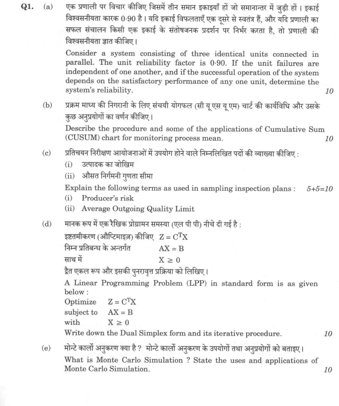
Consider a system consisting of three identical units connected in parallel. The unit reliability factor is 0·90. If the unit failures are independent of one another, and if the successful operation of the system depends on the satisfactory performance of any one unit, determine the system's reliability. 10 marks
Describe the procedure and some of the applications of Cumulative Sum (CUSUM) chart for monitoring process mean. 10 marks
Explain the following terms as used in sampling inspection plans : 5+5=10 marks Producer's risk
Average Outgoing Quality Limit
A Linear Programming Problem (LPP) in standard form is as given below : Optimize Z = CᵀX subject to AX = B with X ≥ 0 Write down the Dual Simplex form and its iterative procedure. 10 marks
What is Monte Carlo Simulation ? State the uses and applications of Monte Carlo Simulation. 10 marks
हिंदी में प्रश्न पढ़ें
एक प्रणाली पर विचार कीजिए जिसमें तीन समान इकाइयाँ हों जो समानान्तर में जुड़ी हों। इकाई विश्वसनीयता कारक 0·90 है। यदि इकाई विफलताएँ एक दूसरे से स्वतंत्र हैं, और यदि प्रणाली का सफल संचालन किसी एक इकाई के संतोषजनक प्रदर्शन पर निर्भर करता है, तो प्रणाली की विश्वसनीयता ज्ञात कीजिए। 10 अंक
प्रक्रम माध्य की निगरानी के लिए संचयी योगफल (सी यू एस यू एम) चार्ट की कार्यविधि और उसके कुछ अनुप्रयोगों का वर्णन कीजिए। 10 अंक
प्रतिचयन निरीक्षण आयोजनाओं में उपयोग होने वाले निम्नलिखित पदों की व्याख्या कीजिए : 5+5=10 अंक उत्पादक का जोखिम
औसत निर्गमी गुणता सीमा
मानक रूप में एक रैखिक प्रोग्रामन समस्या (एल पी पी) नीचे दी गई है : इष्टतमीकरण (ऑप्टिमाइज़) कीजिए Z = CᵀX निम्न प्रतिबन्ध के अन्तर्गत AX = B साथ में X ≥ 0 द्वैत एकल रूप और इसकी पुनरावृत्त प्रक्रिया को लिखिए। 10 अंक
मोंटे कार्लो अनुकरण क्या है ? मोंटे कार्लो अनुकरण के उपयोगों तथा अनुप्रयोगों को बताइए। 10 अंक
Model answer
Written by UPSC Answer Check against this question's marking rubric, to the expected length. UPSC does not publish answers for Mains — this is one way to score well, not an official key.
(a) System Reliability for Three Identical Units in Parallel
When three identical units are connected in parallel and the system succeeds if any one unit operates satisfactorily, the failures are independent and the unit reliability is R = 0.90. The system fails only when all three units fail simultaneously.
Probability that a single unit fails = 1 − 0.90 = 0.10.
Since failures are independent, the probability that all three units fail together is (0.10)³ = 0.001.
Therefore, the reliability of the parallel system is:
R_system = 1 − (1 − R)³ = 1 − (0.10)³ = 1 − 0.001 = 0.999
Thus, the system reliability is 0.999, or 99.9%. This illustrates the redundancy advantage of parallel configuration: even with a modest unit reliability of 0.90, tripling the units in parallel raises system reliability to 99.9%.
(b) Cumulative Sum (CUSUM) Chart: Procedure and Applications
The CUSUM chart is a sequential quality-control tool that accumulates deviations of successive sample statistics from a target value, making it sensitive to small sustained shifts in the process mean.
Procedure. Let the target mean be μ₀ and let x₁, x₂, … be successive sample means (or individual observations). The cumulative sum is defined as:
Sᵢ = Σⱼ₌₁ⁱ (xⱼ − μ₀)
so that Sᵢ = Sᵢ₋₁ + (xᵢ − μ₀). The plotted statistic Sᵢ is charted against sample number i. If the process mean stays at μ₀, the cumulative sum wanders randomly about zero; a drift in the mean makes Sᵢ trend steadily upward or downward.
Two decision procedures are common. In the V-mask method, a V-shaped template is placed with its apex a fixed distance ahead of the latest plotted point, and the process is declared out of control if any previous point falls outside the arms of the V. In the tabular or decision-interval method, two one-sided sums are maintained:
C⁺ᵢ = max[0, C⁺ᵢ₋₁ + (xᵢ − μ₀) − k] C⁻ᵢ = max[0, C⁻ᵢ₋₁ − (xᵢ − μ₀) − k]
where k is the reference value (often half the shift to be detected) and h is the decision interval. An out-of-control signal is given when either C⁺ or C⁻ exceeds h. The parameters k and h are chosen from the desired average run lengths.
Applications. CUSUM charts are widely used in pharmaceutical quality control to monitor tablet weight, potency and dissolution profiles; in component manufacturing, including precision parts for ISRO and defence production, to detect small drifts in dimensions; and in continuous process industries such as chemicals, cement and steel, where small shifts in mean quality characteristics must be caught early.
(c) Terms in Sampling Inspection Plans
(i) Producer's risk. Producer's risk, denoted α, is the probability that a lot of acceptable quality is rejected by the sampling plan. It is the risk of committing a Type I error — rejecting a good lot. It arises because acceptance is based on a sample, not on full inspection, so a lot whose true fraction defective equals the Acceptable Quality Level (AQL) may still yield a sample with more defectives than the acceptance number. By convention, producer's risk is often set at 5%, meaning a lot at AQL quality has at most a 5% chance of rejection. It protects the producer against unfair rejection of satisfactory lots.
(ii) Average Outgoing Quality Limit (AOQL). When rejected lots are subjected to 100% rectifying inspection and defective items are replaced or reworked, the quality of lots leaving the inspection station improves. The Average Outgoing Quality (AOQ) is the expected proportion defective in outgoing lots and is given by:
AOQ = p · Pₐ · (N − n)/N
where p is the incoming fraction defective, Pₐ is the probability of acceptance, N is the lot size and n is the sample size. As p increases, Pₐ falls, so AOQ first rises and then falls, reaching a maximum. This maximum value is the Average Outgoing Quality Limit (AOQL) — the worst average outgoing quality that the plan can produce, regardless of the incoming quality level. It is a key measure of the protection the sampling plan gives to the consumer.
(d) Dual Simplex Form and Iterative Procedure
The given LPP in standard form is:
Optimize Z = CᵀX, subject to AX = B, X ≥ 0.
For the dual simplex method, the problem is first expressed in a form where the objective is maximization and the constraints are equalities with a starting basic solution that is dual feasible but primal infeasible (some bᵢ < 0). The dual simplex form is obtained by writing the problem as:
Maximize Z = CᵀX, subject to AX = B, X ≥ 0,
with the optimality condition of the simplex method (all cⱼ − zⱼ ≤ 0) satisfied at the outset, while the feasibility condition (all basic variables non-negative) is violated.
Iterative procedure.
Step 1: Start with a basic solution that is dual feasible, i.e. all reduced costs cⱼ − zⱼ ≤ 0, but primal infeasible, i.e. at least one basic variable is negative.
Step 2: Leaving variable. Select the basic variable with the most negative value (most negative bᵢ) as the leaving variable.
Step 3: Entering variable. For the row of the leaving variable, compute the ratios of the reduced costs to the corresponding coefficients in that row, considering only coefficients that are negative. Choose the entering variable as the one giving the minimum absolute ratio |(cⱼ − zⱼ)/a_rj| among a_rj < 0. If no a_rj < 0 exists, the problem has no feasible solution.
Step 4: Perform the usual pivot operation to obtain a new basic solution.
Step 5: Check for feasibility. If all basic variables are non-negative, the current solution is optimal for the primal (and feasible for the dual). Otherwise, return to Step 2 and repeat.
The dual simplex method is especially useful when a starting basic solution is dual feasible but not primal feasible, as happens when constraints are of the ≥ type or when the right-hand side changes after an optimal solution has been obtained.
(e) Monte Carlo Simulation: Meaning, Uses and Applications
Monte Carlo simulation is a stochastic numerical technique that models a system by generating random samples from probability distributions and observing the resulting outcomes. Instead of solving a problem analytically, it repeatedly draws random numbers, transforms them into values of the input variables according to their assumed distributions, evaluates the model for each draw, and aggregates the results to estimate probabilities, means, variances or other statistics. Its power lies in handling complex systems with many interacting random variables where closed-form solutions are intractable.
Uses. It is used to estimate integrals and expectations, to assess risk and uncertainty, to study the behaviour of systems under random variation, and to compare alternative designs or policies when analytical methods fail. Accuracy improves as the number of trials increases, typically at a rate proportional to the square root of the number of trials.
Applications. Monte Carlo methods are applied in nuclear shielding design to simulate neutron transport and radiation penetration; in financial risk modelling to value options and estimate Value-at-Risk; in Indian monsoon prediction and climate studies to model rainfall variability; in reliability and queuing analysis; in project management through PERT simulation; and in defence and aerospace for mission reliability assessment. They are also used in inventory control, traffic flow studies and portfolio optimisation.
In summary, the parallel reliability calculation shows how redundancy raises system reliability to 99.9%; the CUSUM chart provides a sensitive sequential procedure for detecting small mean shifts; producer's risk and AOQL quantify the risks borne by producer and consumer in sampling inspection; the dual simplex method offers an efficient algorithm when a dual-feasible but primal-infeasible basis is available; and Monte Carlo simulation provides a versatile stochastic tool for modelling uncertainty across engineering, finance and climate applications.
What "Describe" is asking you to do
Give a full, ordered account of the thing named — its parts, stages or mechanism — in the sequence in which it actually exists or occurs. Most describe questions come from the science optionals, where the marks sit in correct technical detail and, where the stem says so, a labelled diagram.
Structure that answers it
One-line identification of the subject → the parts or stages in their real order, each with its defining detail → labelled diagram where the subject is structural → closing line on function or significance
Where marks are lost
Loose general prose where the examiner is ticking named parts, correct terminology and their sequence; and in the General Studies papers, turning to evaluation before the description is finished.
How this answer will be evaluated
Approach
(a) calculate: given > formula > substitution > result with units > interpretation | (b) describe: define > structure or process in order > labelled diagram > significance | (c(i)) explain: definition/context > points in order > small example > short close | (c(ii)) explain: definition/context > points in order > small example > short close | (d) derive: given > assumptions > stepwise derivation > result > check | (e) explain: definition/context > points in order > small example > short close Full marks: All parts show correct method, clear notation, and contextual interpretation.
Key points expected
- State parallel system reliability formula
- Substitute unit reliability 0.90
- Compute final value 0.999
- Interpret result in context
- Define CUSUM chart
- Explain plotting procedure
- State decision rules
- List at least 2 applications
Evaluation rubric
Each sub-part is marked on its own, against the marks and word limit printed on the paper.
- (a) System reliability for 3 parallel units with p=0.90. 10 marks
calculate— given → formula → substitution → result with units → interpretation
Must cover
- State parallel system reliability formula
- Substitute unit reliability 0.90
- Compute final value 0.999
- Interpret result in context
Loses marks
- Using series formula instead
- No interpretation of result
Earns more
- Explicit independence assumption
- Step-by-step calculation shown
Extra mark
- Comparison with series system
- (b) CUSUM chart procedure and applications for process mean. 10 marks
describe— define → structure or process in order → labelled diagram → significance
Must cover
- Define CUSUM chart
- Explain plotting procedure
- State decision rules
- List at least 2 applications
Loses marks
- Confusing CUSUM with EWMA
- No mention of process mean
Earns more
- Mention of k and h parameters
- Comparison with Shewhart chart
Extra mark
- Worked numerical example
- (c(i)) Definition and context of Producer's risk. 5 marks
explain— definition/context → points in order → small example → short close
Must cover
- Define Producer's risk (α)
- Link to AQL
- Explain probability of rejection
Loses marks
- Confusing with Consumer's risk
- No link to AQL
Earns more
- Mention of OC curve
- Practical implication for producer
Extra mark
- Numerical example of α
- (c(ii)) Definition and significance of AOQL. 5 marks
explain— definition/context → points in order → small example → short close
Must cover
- Define AOQL
- Explain as maximum AQL
- Link to sampling plan
Loses marks
- Confusing with AQL
- No explanation of 'limit'
Earns more
- Mention of 100% inspection effect
- Position on OC curve
Extra mark
- Formula for AOQL
- (d) Dual Simplex form and iterative procedure for LPP. 10 marks
derive— given → assumptions → stepwise derivation → result → check
Must cover
- State dual problem formulation
- Explain dual feasibility condition
- Describe pivot selection rule
- Outline iteration steps
Loses marks
- Confusing with Primal Simplex
- No mention of feasibility
Earns more
- Mention of reduced costs
- Termination condition
Extra mark
- Small numerical example
- (e) Definition, uses, and applications of Monte Carlo Simulation. 10 marks
explain— definition/context → points in order → small example → short close
Must cover
- Define Monte Carlo Simulation
- Explain random sampling principle
- List at least 3 applications
- Mention one use case
Loses marks
- No mention of randomness
- Vague applications
Earns more
- Mention of pseudo-random numbers
- Comparison with analytical methods
Extra mark
- Specific industry example
Practice this exact question
Write your answer and it is marked point by point against the model answer above — what you covered, what you missed, what you got wrong.
Evaluate my answer →More from Statistics 2024 Paper II
- Q1 (a) Consider a system consisting of three identical units connected in parallel. The unit…
- Q2 (a) Obtain the control limits for X̄-chart and R-chart and describe the significance of j…
- Q3 (a) With respect to a given Linear Programming Problem (LPP), explain the following conce…
- Q4 (a) A manually handled toll-booth has two tellers, who are each capable of handling an av…