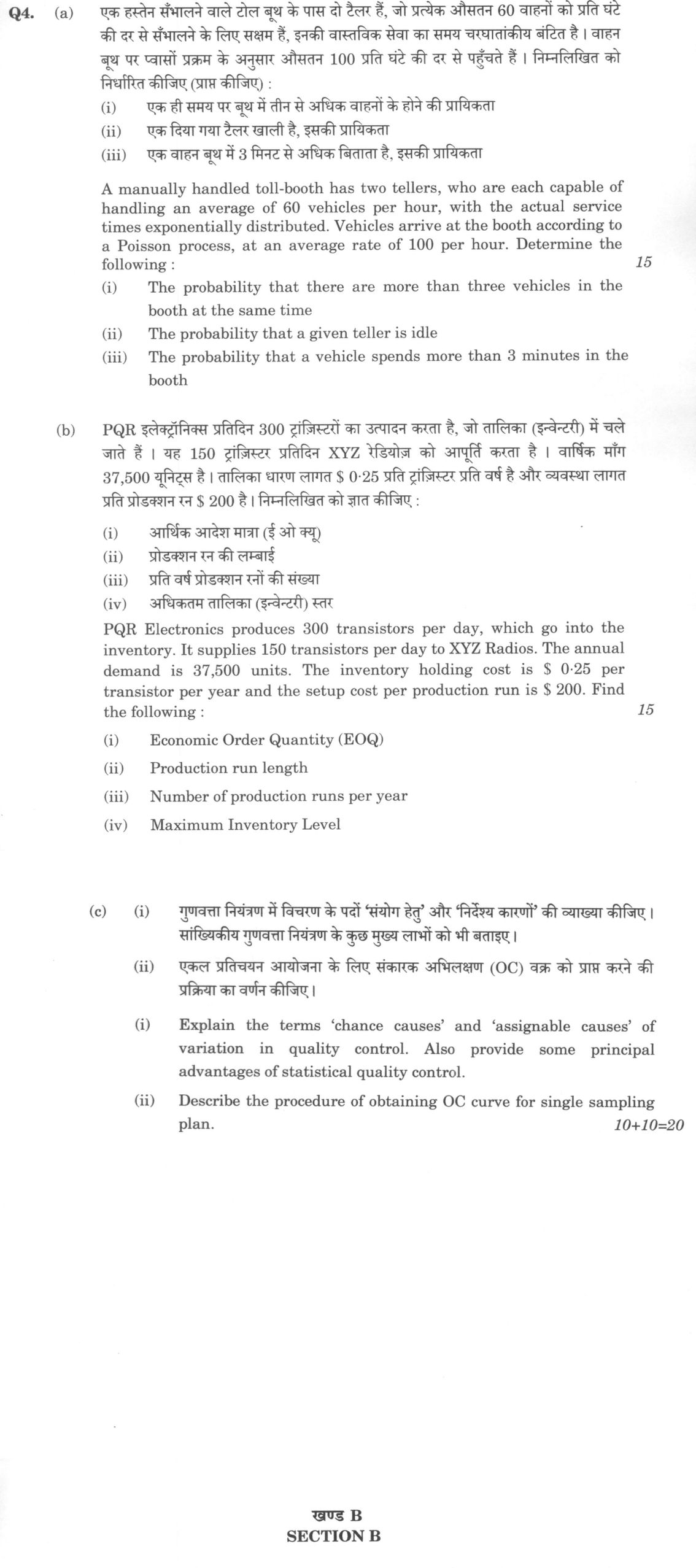
(a) A manually handled toll-booth has two tellers, who are each capable of handling an average of 60 vehicles per hour, with the actual service times exponentially distributed. Vehicles arrive at the booth according to a Poisson process, at an averag

Question

(a) A manually handled toll-booth has two tellers, who are each capable of handling an average of 60 vehicles per hour, with the actual service times exponentially distributed. Vehicles arrive at the booth according to a Poisson process, at an average rate of 100 per hour. Determine the following : 15 marks
(i) The probability that there are more than three vehicles in the booth at the same time
(ii) The probability that a given teller is idle
(iii) The probability that a vehicle spends more than 3 minutes in the booth

(b) PQR Electronics produces 300 transistors per day, which go into the inventory. It supplies 150 transistors per day to XYZ Radios. The annual demand is 37,500 units. The inventory holding cost is 0·25 per transistor per year and the setup cost per production run is 200. Find the following : 15 marks
(i) Economic Order Quantity (EOQ)
(ii) Production run length
(iii) Number of production runs per year
(iv) Maximum Inventory Level

(c) (i) Explain the terms 'chance causes' and 'assignable causes' of variation in quality control. Also provide some principal advantages of statistical quality control. 10 marks
(ii) Describe the procedure of obtaining OC curve for single sampling plan. 10 marks

UPSC Answer Check · Accepted Answer

(a)(i)
This is an M/M/2 queue with λ = 100 vehicles/hour, μ = 60 vehicles/hour per teller, s = 2.
Traffic intensity ρ = λ/(sμ) = 100/(2×60) = 5/6 < 1, so steady state exists.
Using the M/M/2 steady-state probabilities:
P₀ = [Σ (n=0 to 1) (λ/μ)ⁿ/n! + ((λ/μ)²/2!)(1/(1−ρ))]⁻¹.
Here λ/μ = 100/60 = 5/3.
P₀ = [1 + 5/3 + (25/9)/2 × 6]⁻¹ = [1 + 5/3 + 25/3]⁻¹ = 1/11.
P₁ = P₀(5/3) = 5/33.
P₂ = P₀(5/3)²/2! = 25/198.
P₃ = P₂ρ = (25/198)(5/6) = 125/1188.
Therefore,
P(n > 3) = 1 − [1/11 + 5/33 + 25/198 + 125/1188]
= 1 − 563/1188
= 625/1188 ≈ 0.5261.

(a)(ii)
A given teller is idle if either the system is empty, or exactly one vehicle is present and the other teller is serving it. By symmetry:
P(given teller idle) = P₀ + (1/2)P₁
= 1/11 + (1/2)(5/33)
= 1/11 + 5/66
= 11/66
= 1/6 ≈ 0.1667.

(a)(iii)
Let W be total time spent in the booth. For M/M/2,
P(Wq > u) = P(delay) exp(−cμ(1−ρ)u),
where c = 2, μ = 60, ρ = 5/6, so cμ(1−ρ) = 2×60×(1/6) = 20/hour.
Also P(delay) = P(n ≥ 2) = 1 − P₀ − P₁ = 1 − 1/11 − 5/33 = 25/33.
Thus P(Wq > u) = (25/33) exp(−20u).

Service time S is exponential with mean 1/60 hour. For t = 3 minutes = 0.05 hour,
P(W > t) = P(S > t) + ∫₀ᵗ P(Wq > t−s) 60 exp(−60s) ds
= exp(−60t) + (25/22)[exp(−20t) − exp(−60t)].
At t = 0.05:
P(W > 0.05) = (25/22)exp(−1) − (3/22)exp(−3)
= (25e⁻¹ − 3e⁻³)/22 ≈ 0.4113.

(b)
This is the finite-replenishment EOQ/EPQ model.
D = 37,500 units/year, S = 200 per run, H = 0.25 per unit per year.
Since 37,500/150 = 250 working days, d = 150 units/day and p = 300 units/day, so
1 − d/p = 1 − 150/300 = 1/2.

(b)(i)
Q* = √(2DS/[H(1−d/p)])
= √(2×37500×200/[0.25×0.5])
= √(15,000,000/0.125)
= √120,000,000
= 2000√30 ≈ 10,954.45 units.

(b)(ii)
Production run length = Q*/p = 2000√30/300 = (20√30)/3 days ≈ 36.51 days.

(b)(iii)
Number of production runs per year = D/Q*
= 37500/(2000√30)
= 5√30/8 ≈ 3.42 runs/year.

(b)(iv)
Maximum inventory level = Q*(1 − d/p)
= 2000√30 × 1/2
= 1000√30 ≈ 5,477.23 units.

(c)(i)
Chance causes of variation are natural, random, and inherent in a process. They arise from many small uncontrollable sources such as minor vibration, temperature fluctuation, or raw-material variation. They make the process stable but not perfect. A process affected only by chance causes is said to be in statistical control.

Assignable causes of variation are non-random, special causes that can be identified and removed. They arise from specific factors such as machine wear, wrong setting, defective material, operator error, or tool failure. They usually produce large shifts or unusual patterns in quality characteristics. If assignable causes are present, the process is out of control and corrective action is needed.

Principal advantages of statistical quality control are:
Early detection of process shifts before defective items are mass-produced.
Reduction in rework, scrap, inspection cost, and warranty cost.
Scientific acceptance or rejection of lots using sampling plans.
Establishment of quality standards and control limits.
Continuous improvement through diagnosis of assignable causes.
Better productivity, customer satisfaction, and competitive strength.

(c)(ii)
A single sampling plan is specified by lot size N, sample size n, and acceptance number c. From a lot, draw a random sample of n items. If the number of defectives d ≤ c, accept the lot; if d > c, reject it. The OC curve plots Pa(p), the probability of accepting the lot, against p, the fraction defective in the incoming lot.

Procedure:
1. Fix N, n, and c.
2. For a chosen p, compute the probability distribution of d in the sample.
3. If N is finite and sampling is without replacement, use the hypergeometric distribution:
Pa(p) = Σ (x=0 to c) C(Np,x) C(N−Np,n−x)/C(N,n).
4. If N is large compared with n, or the process is effectively infinite, use the binomial distribution:
Pa(p) = Σ (x=0 to c) C(n,x) pˣ (1−p)ⁿ⁻ˣ.
5. If n is large and p is small with np moderate, use the Poisson approximation:
Pa(p) = Σ (x=0 to c) exp(−np)(np)ˣ/x!.
6. Vary p from 0 to 1, or over a practical range, and compute Pa(p) each time.
7. Plot Pa(p) on the vertical axis against p on the horizontal axis and join the points smoothly.
8. The resulting curve starts near Pa = 1 for p = 0, decreases as p increases, and approaches 0 for large p. AQL and LTPD can be marked on it to read producer’s risk α = 1 − Pa(AQL) and consumer’s risk β = Pa(LTPD).

(a) A manually handled toll-booth has two tellers, who are each capable of handling an average of 60 vehicles per hour, with the…

Model answer

What "Solve" is asking you to do

Structure that answers it

Where marks are lost

How this answer will be evaluated

Approach

Key points expected

Evaluation rubric

Must cover

Loses marks

Earns more

Extra mark

Must cover

Loses marks

Earns more

Extra mark

Must cover

Loses marks

Earns more

Extra mark

Must cover

Loses marks

Earns more

Extra mark

Practice this exact question

More from Statistics 2024 Paper II