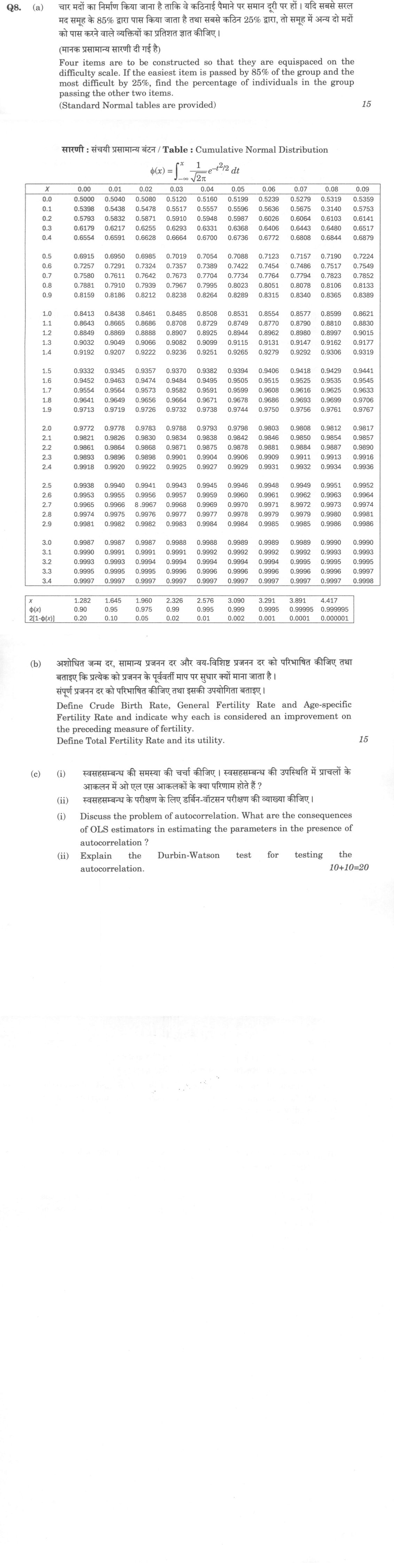
(a) Four items are to be constructed so that they are equispaced on the difficulty scale. If the easiest item is passed by 85% of the group and the most difficult by 25%, find the percentage of individuals in the group passing the other two items.

(

Question

(a)

Four items are to be constructed so that they are equispaced on the difficulty scale. If the easiest item is passed by 85% of the group and the most difficult by 25%, find the percentage of individuals in the group passing the other two items.

(Standard Normal tables are provided) 15 marks

(Standard Normal tables are provided) 15

(b) Define Crude Birth Rate, General Fertility Rate and Age-specific Fertility Rate and indicate why each is considered an improvement on the preceding measure of fertility.

Define Total Fertility Rate and its utility. 15

(c) (i) Discuss the problem of autocorrelation. What are the consequences of OLS estimators in estimating the parameters in the presence of autocorrelation ?

(ii) Explain the Durbin-Watson test for testing the autocorrelation. 10+10=20

UPSC Answer Check · Accepted Answer

(a) In the normal-ogive difficulty model, if p is the proportion passing an item, its difficulty coordinate is z = Φ⁻¹(1−p), since p = P(Z ≥ z). Let the four difficulty coordinates be z₁, z₂, z₃, z₄ in increasing difficulty. Given easiest item: p₁ = 0.85, so z₁ = Φ⁻¹(0.15) = −1.036. Given hardest item: p₄ = 0.25, so z₄ = Φ⁻¹(0.75) = 0.674. Equispacing gives interval h = (z₄ − z₁)/3 = (0.674 − (−1.036))/3 = 1.710/3 = 0.570. Thus z₂ = −1.036 + 0.570 = −0.466, and z₃ = −1.036 + 2(0.570) = 0.104. Therefore p₂ = P(Z ≥ −0.466) = Φ(0.466) = 0.6794 = 67.94%. p₃ = P(Z ≥ 0.104) = 1 − Φ(0.104) = 1 − 0.5415 = 0.4585 = 45.85%. So the other two items are passed by 67.94% and 45.85% respectively, under normality and equal spacing on the normal difficulty scale. (b) Crude Birth Rate (CBR) = (B/P) × 1000, where B is the number of live births in a year and P is mid-year total population. It is “crude” because the denominator includes all persons, many of whom are not exposed to childbearing; it is distorted by age-sex composition. General Fertility Rate (GFR) = (B/W₁₅₋₄₉) × 1000, where W₁₅₋₄₉ is mid-year female population aged 15–49 years. It improves on CBR by relating births only to women of reproductive age, thus removing the effect of males, children and older persons. It is still affected by the age distribution within 15–49. Age-Specific Fertility Rate (ASFR) = (Bₐ/Wₐ) × 1000, where Bₐ is births to women aged a and Wₐ is mid-year female population aged a. It improves on GFR by controlling for age composition; it shows the age pattern and peak of fertility. But it gives many rates rather than one summary index. Total Fertility Rate (TFR) = 5 Σ ASFRᵢ/1000 over five-year age groups 15–19, …, 45–49; for single years, TFR = Σ ASFRₐ/1000. It is the average number of children a woman would bear in a synthetic cohort if current age-specific rates prevailed and she survived through reproductive ages. Its utility is that it gives a single, age-composition-free summary for comparing fertility over time and regions, assessing replacement level (≈2.1), and making population projections. It is a period measure, not actual completed family size, and is affected by timing/tempo changes. (c)(i) Autocorrelation is the violation of Cov(uₜ,uₛ) = 0 for t ≠ s in a regression model yₜ = Xₜβ + uₜ. A common first-order form is uₜ = ρuₜ₋₁ + εₜ, |ρ| < 1, where εₜ is white noise. Causes include inertia, omitted variables, wrong functional form, interpolation, seasonality and lagged variables. Under E(X′u) = 0 and exogenous/nonstochastic regressors, OLS remains unbiased and consistent. But the Gauss-Markov theorem fails, so OLS is not BLUE. The true variance is Var(b) = σ²(X′X)⁻¹X′ΩX(X′X)⁻¹, not σ²(X′X)⁻¹. Hence usual OLS standard errors, t, F and confidence intervals are invalid. With positive autocorrelation, standard errors are often understated, causing spurious significance. OLS is inefficient and forecasts/tests become unreliable. If lagged dependent variables are present with autocorrelated errors, OLS becomes biased and inconsistent. Remedies include GLS, Cochrane-Orcutt/Prais-Winsten, or HAC/Newey-West standard errors. (c)(ii) The Durbin-Watson test tests first-order autocorrelation. Fit OLS and obtain residuals eₜ. The statistic is d = [Σₜ₌₂ⁿ (eₜ − eₜ₋₁)²] / [Σₜ₌₁ⁿ eₜ²]. For large n, d ≈ 2(1 − r), where r = Σₜ₌₂ⁿ eₜeₜ₋₁ / Σₜ₌₁ⁿ eₜ². Hence 0 ≤ d ≤ 4; d ≈ 2 means no autocorrelation, d < 2 indicates positive autocorrelation, and d > 2 indicates negative autocorrelation. Null H₀: ρ = 0. Tables give lower d_L and upper d_U for given n, number of regressors k (excluding intercept), and significance level. For H₁: ρ > 0, if d < d_L reject H₀; if d > d_U do not reject; if d_L ≤ d ≤ d_U the result is inconclusive. For negative autocorrelation, compare 4 − d with d_L and d_U: if 4 − d < d_L (i.e. d > 4 − d_L), reject H₀; if 4 − d > d_U (i.e. d < 4 − d_U), do not reject; otherwise inconclusive. The test assumes an intercept, nonstochastic regressors, no lagged dependent variable, first-order AR errors, and normally distributed errors for exact inference; it cannot detect higher-order autocorrelation. With lagged dependent variables, use Durbin h or Breusch-Godfrey.

(a) Four items are to be constructed so that they are equispaced on the difficulty scale. If the easiest item is passed by 85% of…

Model answer

What "Solve" is asking you to do

Structure that answers it

Where marks are lost

How this answer will be evaluated

Approach

Key points expected

Evaluation rubric

Must cover

Loses marks

Earns more

Extra mark

Must cover

Loses marks

Earns more

Extra mark

Must cover

Loses marks

Earns more

Extra mark

Must cover

Loses marks

Earns more

Extra mark

Practice this exact question

More from Statistics 2024 Paper II