Paper II — Q3
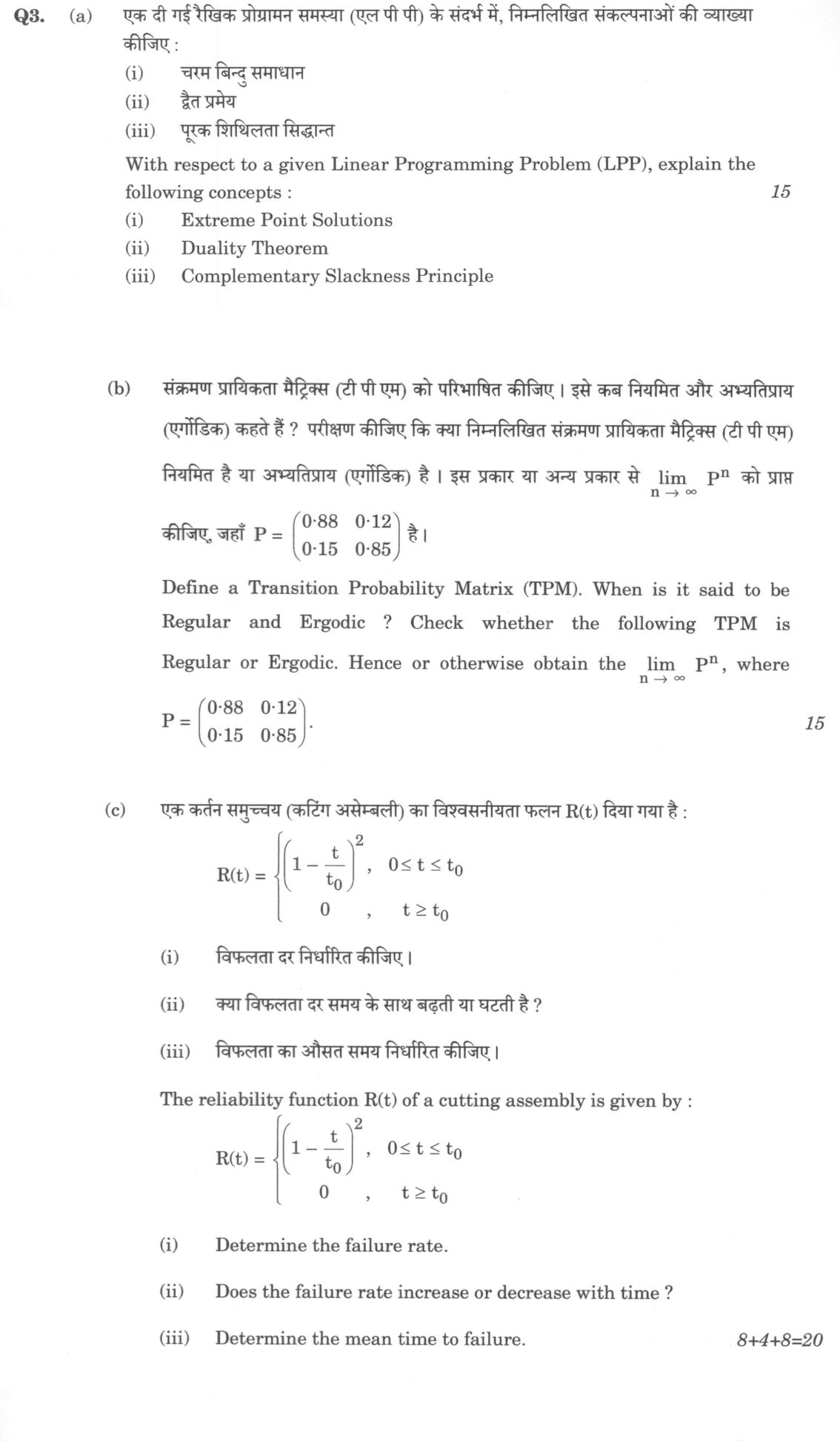
(a) With respect to a given Linear Programming Problem (LPP), explain the following concepts : 15 marks (i) Extreme Point…
With respect to a given Linear Programming Problem (LPP), explain the following concepts : 15 marks Extreme Point Solutions
Duality Theorem
Complementary Slackness Principle
Define a Transition Probability Matrix (TPM). When is it said to be Regular and Ergodic ? Check whether the following TPM is Regular or Ergodic. Hence or otherwise obtain the limlimitsₙ → ∞ Pⁿ, where P = 0.88 & 0.12 0.15 & 0.85 . 15 marks
The reliability function R(t) of a cutting assembly is given by : R(t) = (1-t/(t₀))², & 0 ≤ t ≤ t₀ 0 & , t ≥ t₀ Determine the failure rate.
Does the failure rate increase or decrease with time ?
Determine the mean time to failure. 8+4+8=20 marks
हिंदी में प्रश्न पढ़ें
एक दी गई रैखिक प्रोग्रामन समस्या (एल पी पी) के संदर्भ में, निम्नलिखित संकल्पनाओं की व्याख्या कीजिए : 15 अंक चरम बिन्दु समाधान
द्वैत प्रमेय
पूरक शिथिलता सिद्धांत
संक्रमण प्रायिकता मैट्रिक्स (टी पी एम) को परिभाषित कीजिए। इसे कब नियमित और अभ्यतिग्राय (एर्गोडिक) कहते हैं ? परीक्षण कीजिए कि क्या निम्नलिखित संक्रमण प्रायिकता मैट्रिक्स (टी पी एम) नियमित है या अभ्यतिग्राय (एर्गोडिक) है। इस प्रकार या अन्य प्रकार से limlimitsₙ → ∞ Pⁿ को प्राप्त कीजिए, जहाँ P = 0.88 & 0.12 0.15 & 0.85 है। 15 अंक
एक कतन समुच्चय (कटिंग असेंबली) का विश्वसनीयता फलन R(t) दिया गया है : R(t) = (1-t/(t₀))², & 0 ≤ t ≤ t₀ 0 & , t ≥ t₀ विफलता दर निर्धारित कीजिए।
क्या विफलता दर समय के साथ बढ़ती या घटती है ?
विफलता का औसत समय निर्धारित कीजिए। 8+4+8=20 अंक
Model answer
Written by UPSC Answer Check against this question's marking rubric, to the expected length. UPSC does not publish answers for Mains — this is one way to score well, not an official key.
(a) Concepts in Linear Programming
(i) Extreme Point Solutions In an LPP, the feasible region defined by the constraints is a convex polyhedron. A feasible solution is an extreme point (vertex) if it cannot be expressed as a strict convex combination of two other distinct feasible solutions, i.e. it lies at a corner where at least n linearly independent constraints intersect (n being the number of variables). The Fundamental Theorem of LPP states that if an optimal solution exists, at least one optimal solution occurs at an extreme point, because a linear objective function attains its maximum/minimum over a convex polytope at a vertex. This is why the simplex method searches only among basic feasible solutions (extreme points) rather than the infinite feasible set.
(ii) Duality Theorem Every primal LPP has an associated dual. Weak duality states that for any feasible primal x and dual y, the primal objective ≤ dual objective (for maximisation primal). Strong duality states that if either problem has a finite optimal solution, so does the other, and their optimal objective values are equal. The dual variables are shadow prices: they measure the marginal change in the optimal objective per unit relaxation of a constraint, giving the economic worth of scarce resources.
(iii) Complementary Slackness Principle At optimality, for each primal constraint, the product of its slack and the corresponding dual variable is zero; similarly for each dual constraint, the product of its surplus and the corresponding primal variable is zero. Thus a resource with positive slack (not fully used) has zero shadow price, and a resource with positive shadow price is fully exhausted. It is a powerful optimality-verification tool.
(b) Transition Probability Matrix A TPM P = [p_ij] gives the one-step transition probabilities of a Markov chain, satisfying p_ij ≥ 0 and each row summing to 1 (row-stochastic). A chain is Regular if some power Pⁿ has all entries strictly positive. It is Ergodic if it is irreducible (all states communicate) and aperiodic; a regular chain is ergodic.
For P = [[0.88,0.12],[0.15,0.85]], all entries are positive, so P itself has all positive entries; hence P is regular and ergodic. The limiting distribution π satisfies πP = π, π₁+π₂=1: 0.88π₁+0.15π₂ = π₁ → 0.15π₂ = 0.12π₁ → π₁/π₂ = 5/4. With π₁+π₂=1: π = (5/9, 4/9). Hence lim Pⁿ has both rows equal to (5/9, 4/9).
(c) Reliability Function R(t) = (1 − t/t₀)², 0 ≤ t ≤ t₀; 0 for t ≥ t₀.
(i) Failure rate: λ(t) = −R′(t)/R(t). R′(t) = −(2/t₀)(1 − t/t₀). So λ(t) = [(2/t₀)(1 − t/t₀)] / (1 − t/t₀)² = 2/(t₀ − t), for 0 ≤ t < t₀.
(ii) Monotonicity: λ′(t) = 2/(t₀ − t)² > 0, so the failure rate increases with time — an Increasing Failure Rate (IFR) distribution, characteristic of a wear-out phase.
(iii) MTTF: MTTF = ∫₀^t₀ R(t)dt = ∫₀^t₀(1 − t/t₀)²dt. Let u = 1 − t/t₀, dt = −t₀du: = t₀∫₀¹u²du = t₀/3.
Thus the assembly has an increasing failure rate and a mean life of one-third of its maximum support t₀.
What "Explain" is asking you to do
Make the working of something clear — what sets it off, what follows from what, and what it produces. Explain is the Commission's mechanism word: it dominates the technical papers and the “explain why” stems, where the marks sit in the causal chain and not in the label.
Structure that answers it
State what it is → the initiating condition → the chain of cause, step by step → an instance where it plays out → what the chain produces
Where marks are lost
Describing what something looks like instead of why it works that way. Naming the stages without linking them reads as description too.
How this answer will be evaluated
Approach
(a) explain: definition/context > points in order > small example > short close | (b) define: precise definition > the distinguishing feature > one example | (c(i)) calculate: given > formula > substitution > result with units > interpretation | (c(ii)) comment: context > arguments both sides > judgment > close | (c(iii)) calculate: given > formula > substitution > result with units > interpretation Full marks: All parts fully answered with correct derivations, clear definitions, and proper interpretation.
Key points expected
- Define Extreme Point Solutions as vertices of feasible region
- State Duality Theorem linking primal and dual optimal values
- State Complementary Slackness Principle conditions for optimality
- Provide a small example or context for each concept
- Define TPM with row-stochastic property
- Define Regular (some power has all positive entries)
- Define Ergodic (unique stationary distribution)
- Calculate limit P^n as n approaches infinity
Evaluation rubric
Each sub-part is marked on its own, against the marks and word limit printed on the paper.
- (a) Define and explain three specific LPP concepts. 15 marks
explain— definition/context → points in order → small example → short close
Must cover
- Define Extreme Point Solutions as vertices of feasible region
- State Duality Theorem linking primal and dual optimal values
- State Complementary Slackness Principle conditions for optimality
- Provide a small example or context for each concept
Loses marks
- Confusing extreme points with basic feasible solutions
- Stating duality without mentioning optimality conditions
- Omitting the 'slackness' condition in complementary slackness
Earns more
- Mention geometric interpretation of extreme points
- Note strong duality theorem specifically
- Show algebraic form of complementary slackness
Extra mark
- Reference to Simplex method for finding extreme points
- Mention sensitivity analysis in context of duality
- (b) Define TPM, Regular/Ergodic, classify given matrix, find limit. 15 marks
define— precise definition → the distinguishing feature → one example
Must cover
- Define TPM with row-stochastic property
- Define Regular (some power has all positive entries)
- Define Ergodic (unique stationary distribution)
- Calculate limit P^n as n approaches infinity
Loses marks
- Confusing Regular with Irreducible
- Failing to check if the given matrix is regular
- Incorrect calculation of the limit matrix
Earns more
- Show calculation of stationary distribution vector
- Verify regularity by checking P^2 or P^k
- State that regular implies ergodic for finite chains
Extra mark
- Mention Perron-Frobenius theorem
- Provide a diagram of the state transition graph
- (c(i)) Determine the failure rate function from R(t). 8 marks
calculate— given → formula → substitution → result with units → interpretation
Must cover
- State formula for failure rate h(t) = -R'(t)/R(t)
- Differentiate R(t) = (1 - t/t0)^2
- Substitute into formula to find h(t)
- Simplify to h(t) = 2/(t0 - t)
Loses marks
- Using h(t) = f(t)/R(t) without deriving f(t)
- Sign error in derivative of R(t)
- Failing to simplify the final expression
Earns more
- Show step-by-step differentiation
- State domain of validity 0 <= t < t0
Extra mark
- Mention units of failure rate (per time unit)
- (c(ii)) State if failure rate increases or decreases with time. 4 marks
comment— context → arguments both sides → judgment → close
Must cover
- Analyze h(t) = 2/(t0 - t) for t in [0, t0)
- State that h(t) increases as t increases
- Justify by noting denominator decreases as t increases
Loses marks
- Stating 'decreases' without justification
- Confusing failure rate with reliability function
Earns more
- Mention this is an increasing failure rate (IFR) distribution
- Relate to wear-out phase of bathtub curve
Extra mark
- Sketch the shape of the h(t) curve
- (c(iii)) Determine the mean time to failure (MTTF). 8 marks
calculate— given → formula → substitution → result with units → interpretation
Must cover
- State formula MTTF = integral of R(t) from 0 to infinity
- Set up integral of (1 - t/t0)^2 from 0 to t0
- Perform integration to get t0/3
- State final answer with units
Loses marks
- Integrating from 0 to infinity without splitting at t0
- Arithmetic error in integration
- Forgetting to square the term before integrating
Earns more
- Show substitution u = 1 - t/t0 for integration
- Verify result using alternative method if possible
Extra mark
- Mention that MTTF is the first moment of failure time
Practice this exact question
Write your answer and it is marked point by point against the model answer above — what you covered, what you missed, what you got wrong.
Evaluate my answer →More from Statistics 2024 Paper II
- Q1 (a) Consider a system consisting of three identical units connected in parallel. The unit…
- Q2 (a) Obtain the control limits for X̄-chart and R-chart and describe the significance of j…
- Q3 (a) With respect to a given Linear Programming Problem (LPP), explain the following conce…
- Q4 (a) A manually handled toll-booth has two tellers, who are each capable of handling an av…
- Q5 (a) Discuss the Indian Statistical System. State some important organisations and explain…
- Q6 (a) For the linear model Y = Xβ + u, obtain the expressions for Ordinary Least Squares (O…