Paper I — Q5
(a) For a two variable linear regression model Yᵢ = a + bXᵢ + eᵢ, where E(eᵢ) = 0, Var(eᵢ) = σ²ₑ, Cov(eᵢ, eⱼ) = 0 for i ≠ j…
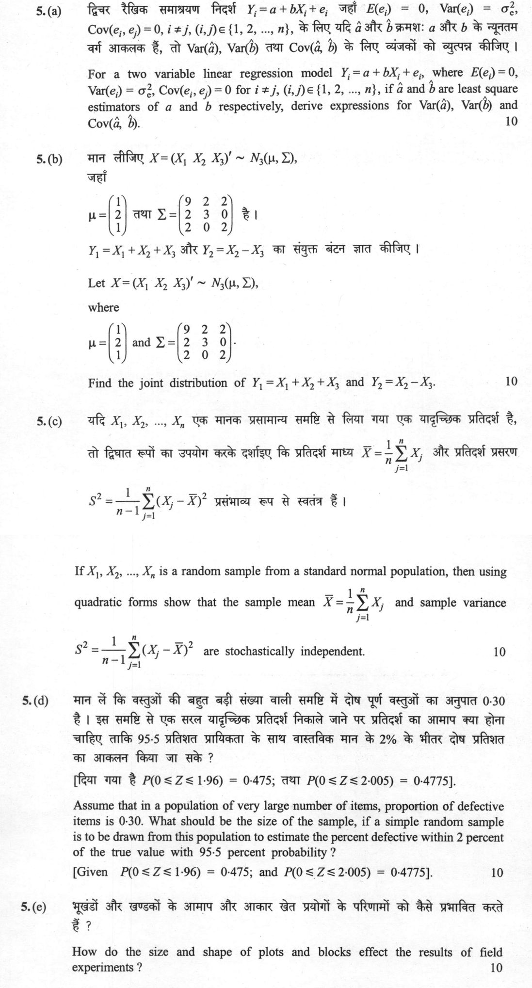
For a two variable linear regression model Yᵢ = a + bXᵢ + eᵢ, where E(eᵢ) = 0, Var(eᵢ) = σ²ₑ, Cov(eᵢ, eⱼ) = 0 for i ≠ j, (i,j) ∈ {1, 2, ..., n}, if â and b̂ are least square estimators of a and b respectively, derive expressions for Var(â), Var(b̂) and Cov(â, b̂). 10 marks
Let X = (X₁ X₂ X₃)' ~ N₃(μ, Σ), where μ = (1 2 1)' and Σ = (9 2 2 / 2 3 0 / 2 0 2). Find the joint distribution of Y₁ = X₁ + X₂ + X₃ and Y₂ = X₂ - X₃. 10 marks
If X₁, X₂, ..., Xₙ is a random sample from a standard normal population, then using quadratic forms show that the sample mean X̄ = (1/n)∑ⱼ₌₁ⁿ Xⱼ and sample variance S² = [1/(n-1)]∑ⱼ₌₁ⁿ(Xⱼ - X̄)² are stochastically independent. 10 marks
Assume that in a population of very large number of items, proportion of defective items is 0·30. What should be the size of the sample, if a simple random sample is to be drawn from this population to estimate the percent defective within 2 percent of the true value with 95·5 percent probability? [Given P(0 ≤ Z ≤ 1·96) = 0·475; and P(0 ≤ Z ≤ 2·005) = 0·4775]. 10 marks
How do the size and shape of plots and blocks effect the results of field experiments? 10 marks
हिंदी में प्रश्न पढ़ें
द्विचर रैखिक समाश्रयन निदर्श Yᵢ = a + bXᵢ + eᵢ जहाँ E(eᵢ) = 0, Var(eᵢ) = σ²ₑ, Cov(eᵢ, eⱼ) = 0, i ≠ j, (i,j) ∈ {1, 2, ..., n}, के लिए यदि â और b̂ क्रमशः a और b के न्यूनतम वर्ग आकलक हैं, तो Var(â), Var(b̂) तथा Cov(â, b̂) के लिए व्यंजकों को व्युत्पन्न कीजिए। 10 अंक
मान लीजिए X = (X₁ X₂ X₃)' ~ N₃(μ, Σ), जहाँ μ = (1 2 1)' तथा Σ = (9 2 2 / 2 3 0 / 2 0 2) है। Y₁ = X₁ + X₂ + X₃ और Y₂ = X₂ - X₃ का संयुक्त बंटन ज्ञात कीजिए। 10 अंक
यदि X₁, X₂, ..., Xₙ एक मानक प्रसामान्य समष्टि से लिया गया एक यादृच्छिक प्रतिदर्श है, तो द्विघात रूपों का उपयोग करके दर्शाइए कि प्रतिदर्श माध्य X̄ = (1/n)∑ⱼ₌₁ⁿ Xⱼ और प्रतिदर्श प्रसरण S² = [1/(n-1)]∑ⱼ₌₁ⁿ(Xⱼ - X̄)² प्रसामान्य रूप से स्वतंत्र हैं। 10 अंक
मान लें कि वस्तुओं की बहुत बड़ी संख्या वाली समष्टि में दोष पूर्ण वस्तुओं का अनुपात 0·30 है। इस समष्टि से एक सरल यादृच्छिक प्रतिदर्श निकाले जाने पर प्रतिदर्श का आमाप क्या होना चाहिए ताकि 95·5 प्रतिशत प्रायिकता के साथ वास्तविक मान के 2% के भीतर दोष प्रतिशत का आकलन किया जा सके? [दिया गया है P(0 ≤ Z ≤ 1·96) = 0·475; तथा P(0 ≤ Z ≤ 2·005) = 0·4775]। 10 अंक
भूखंडों और खंडकों के आमाप और आकार खेत प्रयोगों के परिणामों को कैसे प्रभावित करते हैं? 10 अंक
Model answer
Written by UPSC Answer Check against this question's marking rubric, to the expected length. UPSC does not publish answers for Mains — this is one way to score well, not an official key.
(a) For given X-values, set xᵢ = Xᵢ - X̄ and Sₓₓ = ∑(Xᵢ - X̄)² = ∑xᵢ². The least-squares normal equations are
nâ + b̂∑Xᵢ = ∑Yᵢ,
â∑Xᵢ + b̂∑Xᵢ² = ∑XᵢYᵢ.
Solving them gives
b̂ = ∑(Xᵢ - X̄)(Yᵢ - Ȳ)/Sₓₓ = ∑xᵢYᵢ/Sₓₓ,
and
â = Ȳ - b̂X̄.
Substitute Yᵢ = a + bXᵢ + eᵢ. Since ∑xᵢ = 0,
∑xᵢYᵢ = a∑xᵢ + b∑xᵢXᵢ + ∑xᵢeᵢ = bSₓₓ + ∑xᵢeᵢ.
Hence
b̂ - b = ∑xᵢeᵢ/Sₓₓ.
Therefore
Var(b̂) = E[(∑xᵢeᵢ)²]/Sₓₓ² = σ²ₑ∑xᵢ²/Sₓₓ² = σ²ₑ/Sₓₓ.
For the intercept, Ȳ = a + bX̄ + ē, so
â - a = ē - X̄(b̂ - b) = ∑[1/n - X̄xᵢ/Sₓₓ]eᵢ.
Let cᵢ = 1/n - X̄xᵢ/Sₓₓ. Then
Var(â) = σ²ₑ∑cᵢ².
Now
∑cᵢ² = ∑[1/n² - 2X̄xᵢ/(nSₓₓ) + X̄²xᵢ²/Sₓₓ²] = 1/n - 0 + X̄²/Sₓₓ = 1/n + X̄²/Sₓₓ.
Thus
Var(â) = σ²ₑ(1/n + X̄²/Sₓₓ) = σ²ₑ∑Xᵢ²/(nSₓₓ).
For the covariance, write b̂ - b = ∑dᵢeᵢ with dᵢ = xᵢ/Sₓₓ. Then
Cov(â, b̂) = Cov(∑cᵢeᵢ, ∑dᵢeᵢ) = σ²ₑ∑cᵢdᵢ.
But
∑cᵢdᵢ = ∑[(1/n - X̄xᵢ/Sₓₓ)(xᵢ/Sₓₓ)] = (1/(nSₓₓ))∑xᵢ - (X̄/Sₓₓ²)∑xᵢ² = 0 - X̄/Sₓₓ = -X̄/Sₓₓ.
Hence
Var(b̂) = σ²ₑ/Sₓₓ, Var(â) = σ²ₑ(1/n + X̄²/Sₓₓ), Cov(â, b̂) = -σ²ₑX̄/Sₓₓ.
The result requires Sₓₓ > 0 and the stated uncorrelated, homoscedastic error assumptions.
(b) Let Y = (Y₁, Y₂)' and define the linear transformation
Y₁ = X₁ + X₂ + X₃, Y₂ = X₂ - X₃.
So Y = AX, where
A = [[1, 1, 1], [0, 1, -1]].
Since X ~ N₃(μ, Σ), any linear transformation is normal:
Y ~ N₂(Aμ, AΣA').
Now μ = (1, 2, 1)', so
Aμ = (1 + 2 + 1, 2 - 1)' = (4, 1)'.
Also Σ = [[9, 2, 2], [2, 3, 0], [2, 0, 2]].
Compute the variances:
Var(Y₁) = Var(X₁ + X₂ + X₃) = 9 + 3 + 2 + 2(2) + 2(2) + 2(0) = 22.
Var(Y₂) = Var(X₂ - X₃) = 3 + 2 - 2(0) = 5.
Cov(Y₁, Y₂) = Cov(X₁ + X₂ + X₃, X₂ - X₃) = Cov(X₁, X₂) - Cov(X₁, X₃) + Var(X₂) - Cov(X₂, X₃) + Cov(X₃, X₂) - Var(X₃) = 2 - 2 + 3 - 0 + 0 - 2 = 1.
Therefore
(Y₁, Y₂)' ~ N₂((4, 1)', [[22, 1], [1, 5]]).
Equivalently, Y₁ ~ N(4, 22), Y₂ ~ N(1, 5), and Cov(Y₁, Y₂) = 1.
(c) Let X = (X₁, X₂, ..., Xₙ)' ~ Nₙ(0, I). Put 1 = (1, 1, ..., 1)'. The sample mean is
X̄ = (1/n)1'X.
Define
B = I - (1/n)11'.
Then B is symmetric and idempotent, B² = B, and B1 = 0. Also,
∑ⱼ₌₁ⁿ(Xⱼ - X̄)² = X'X - nX̄² = X'X - (1/n)X'11'X = X'[I - (1/n)11']X = X'BX.
Hence
S² = (1/(n-1))∑(Xⱼ - X̄)² = X'BX/(n-1).
Now consider the scalar L = 1'X and the vector Z = BX. They are jointly normal because both are linear transforms of X. Their covariance is
Cov(L, Z) = Cov(1'X, BX) = 1' Var(X) B' = 1'B = (B1)' = 0.
Thus L and Z are independent, since zero covariance implies independence for jointly normal variables. Therefore X̄ = L/n is independent of Z. But S² = Z'Z/(n-1) is a function of Z. Hence
X̄ and S² are stochastically independent.
Equivalently, by the normal quadratic-form theorem, the idempotent matrices J/n and I - J/n have zero product, so X'(J/n)X and X'[I - J/n]X are independent; these determine X̄² and S², and the sign of X̄ is independent of S² as shown by the linear-form argument.
(d) Let p = 0.30 be the population proportion of defectives and q = 1 - p = 0.70. The phrase “within 2 percent of the true value” means a relative error:
|p̂ - p| ≤ 0.02p.
Thus the permissible absolute error is
e = 0.02p = 0.02 × 0.30 = 0.006.
For a large simple random sample,
p̂ ~ N(p, pq/n).
We require
P(|p̂ - p| ≤ e) = 0.955.
Standardize:
Z = (p̂ - p)/√(pq/n).
Then
P(|Z| ≤ z) = 0.955,
so
P(0 ≤ Z ≤ z) = 0.4775.
The given value gives z = 2.005. Now
z = e/√(pq/n) = e√n/√(pq).
Therefore
n = z²pq/e².
Substitute:
n = (2.005)²(0.30)(0.70)/(0.006)² = (4.020025)(0.21)/0.000036 = 0.84420525/0.000036 = 23450.145833.
Rounding up to the next integer,
n = 23451.
Since the population is very large, the finite-population correction is negligible. The normal approximation is valid because np and nq are large.
If “within 2 percent” were instead interpreted as an absolute margin of 2 percentage points, the corresponding size would be 2111.
(e) The size and shape of plots and blocks strongly affect the precision and validity of field experiments because they determine how much soil heterogeneity, border effect, competition, and management variation enters the experimental error.
For plot size, larger plots generally reduce border effects, interplot competition, and the relative influence of soil micro-variation. They give more representative yields, especially for crops with spreading roots or mobile pests. However, increasing plot size increases total variance per plot and cost, and it may reduce the number of replications for a fixed area. Very small plots are economical and allow more replication, but they suffer more from border effects, damage, missing plants, and treatment interference. The optimum plot size is usually studied by uniformity trials; variance per unit area decreases with plot size at a diminishing rate, so beyond a point the gain in precision is small.
For plot shape, long narrow rectangular plots are often more efficient than square plots because they sample soil heterogeneity better and reduce the correlation between adjacent plots. Their orientation should be chosen with respect to the fertility gradient, usually so that each plot is as representative as possible and block-to-block variation is minimized. Square or compact plots reduce perimeter and border effects, so the best shape depends on the crop and the pattern of soil variation.
For blocks, blocks should be compact and homogeneous so that variation within a block is small relative to variation between blocks. If a fertility gradient is known, blocks are usually laid out perpendicular to that gradient. Large blocks contain more heterogeneity and inflate experimental error; very small blocks may not provide enough error degrees of freedom and can create practical difficulties. The number and shape of plots within a block should balance precision, error degrees of freedom, and field layout. Thus careful choice of plot and block size and shape reduces experimental error and makes treatment comparisons more reliable.
What "Derive" is asking you to do
Reach the stated expression from a starting relation, justifying every step. The destination is printed in the question, so only the route earns marks, and the assumptions you work under are part of that route.
Structure that answers it
Assumptions and notation defined → starting relation or governing equation → each step with its justification → the required expression → limiting case or boundary check
Where marks are lost
Writing the standard result first and fitting three lines to it, which an examiner reads at a glance. Marks also go on assumptions left unstated — lossless medium, small amplitude, errors independent with zero mean — and on symbols used before they are defined, even when the question says usual notations.
How this answer will be evaluated
Approach
(a) derive: given > assumptions > stepwise derivation > result > check | (b) calculate: given > formula > substitution > result with units > interpretation | (c) derive: given > assumptions > stepwise derivation > result > check | (d) calculate: given > formula > substitution > result with units > interpretation | (e) discuss: intro > 3-4 dimensions > example > balanced close Full marks: Complete derivations with all steps, correct calculations, clear interpretation, proper notation throughout
Key points expected
- State OLS normal equations for â and b̂
- Express estimators as linear combinations of Y_i
- Apply Var and Cov properties to linear forms
- State final expressions for Var(â), Var(b̂), Cov(â, b̂)
- Define transformation matrix A for Y = AX
- Calculate mean vector μ_Y = Aμ
- Calculate covariance matrix Σ_Y = AΣA'
- State joint distribution as N₂(μ_Y, Σ_Y)
Evaluation rubric
Each sub-part is marked on its own, against the marks and word limit printed on the paper.
- (a) Derive variance and covariance expressions for OLS estimators in simple linear regression. 10 marks
derive— given → assumptions → stepwise derivation → result → check
Must cover
- State OLS normal equations for â and b̂
- Express estimators as linear combinations of Y_i
- Apply Var and Cov properties to linear forms
- State final expressions for Var(â), Var(b̂), Cov(â, b̂)
Loses marks
- Skipping derivation steps to jump to final formula
- Confusing population parameters with sample estimators
- Incorrect application of variance properties
Earns more
- Explicitly use E(e_i)=0 and Var(e_i)=σ_e²
- Show intermediate algebraic steps clearly
- Correct notation distinguishing estimator from parameter
Extra mark
- Mention Gauss-Markov theorem context
- (b) Find joint distribution of linear combinations of multivariate normal variables. 10 marks
calculate— given → formula → substitution → result with units → interpretation
Must cover
- Define transformation matrix A for Y = AX
- Calculate mean vector μ_Y = Aμ
- Calculate covariance matrix Σ_Y = AΣA'
- State joint distribution as N₂(μ_Y, Σ_Y)
Loses marks
- Incorrect matrix multiplication
- Failing to state the distribution type
- Arithmetic errors in mean or covariance calculation
Earns more
- Correct matrix multiplication steps shown
- Explicitly state that linear combinations of MVN are MVN
- Clean presentation of matrix operations
Extra mark
- Verify positive definiteness of resulting covariance matrix
- (c) Prove stochastic independence of sample mean and variance using quadratic forms. 10 marks
derive— given → assumptions → stepwise derivation → result → check
Must cover
- Express X̄ and S² as quadratic forms in X
- Identify idempotent matrices P and Q
- Show PQ = 0 (orthogonality condition)
- Apply theorem: independent if PQ=0 for normal variables
Loses marks
- Failing to show PQ=0 condition
- Incorrect matrix representation of quadratic forms
- Skipping the theorem statement
Earns more
- Correct identification of projection matrices
- Clear statement of the quadratic form independence theorem
- Proper notation for sample mean and variance
Extra mark
- Mention degrees of freedom for each quadratic form
- (d) Calculate sample size for estimating proportion with specified precision and confidence. 10 marks
calculate— given → formula → substitution → result with units → interpretation
Must cover
- State formula n = (Z²pq)/d²
- Identify p=0.30, q=0.70, d=0.02
- Determine Z-value from given probability 0.4775
- Calculate and interpret final sample size
Loses marks
- Using wrong Z-value (1.96 instead of 2.005)
- Arithmetic errors in calculation
- Failing to interpret the sample size
Earns more
- Correct identification of Z=2.005 from given data
- Clear substitution steps shown
- Interpretation of result in context
Extra mark
- Mention finite population correction if applicable
- (e) Discuss how plot and block size/shape affect field experiment results. 10 marks
discuss— intro → 3-4 dimensions → example → balanced close
Must cover
- Explain effect of plot size on experimental error
- Discuss block size and shape on heterogeneity control
- Mention edge effects and their mitigation
- Provide balanced conclusion on optimal design
Loses marks
- Vague general statements without specific effects
- Ignoring one of size or shape
- No practical examples or context
Earns more
- Specific examples of size/shape effects
- Mention of rectangular vs square plots
- Reference to practical field constraints
Extra mark
- Mention of specific experimental designs (RCBD, etc.)
Practice this exact question
Write your answer and it is marked point by point against the model answer above — what you covered, what you missed, what you got wrong.
Evaluate my answer →More from Statistics 2025 Paper I
- Q2 (a) Let X be a continuous random variable having probability density function f(x) = (2/2…
- Q3 (a) Let probability of obtaining Head on a biased coin be 4/5 and X be the number of head…
- Q4 (a) Let X₁, X₂, ... be a sequence of random variables from Bernoulli distribution with me…
- Q5 (a) For a two variable linear regression model Yᵢ = a + bXᵢ + eᵢ, where E(eᵢ) = 0, Var(eᵢ…
- Q6 (a)(i) If (X, Y) follows bivariate normal BN(μ₁, μ₂, σ₁², σ₂², ρ), then obtain (A) E(e^X)…
- Q7 (a) Analyse and interpret the following data concerning output of wheat per field obtaine…
- Q8 (a)(i) What are principal components ? Show that the principal components are uncorrelate…