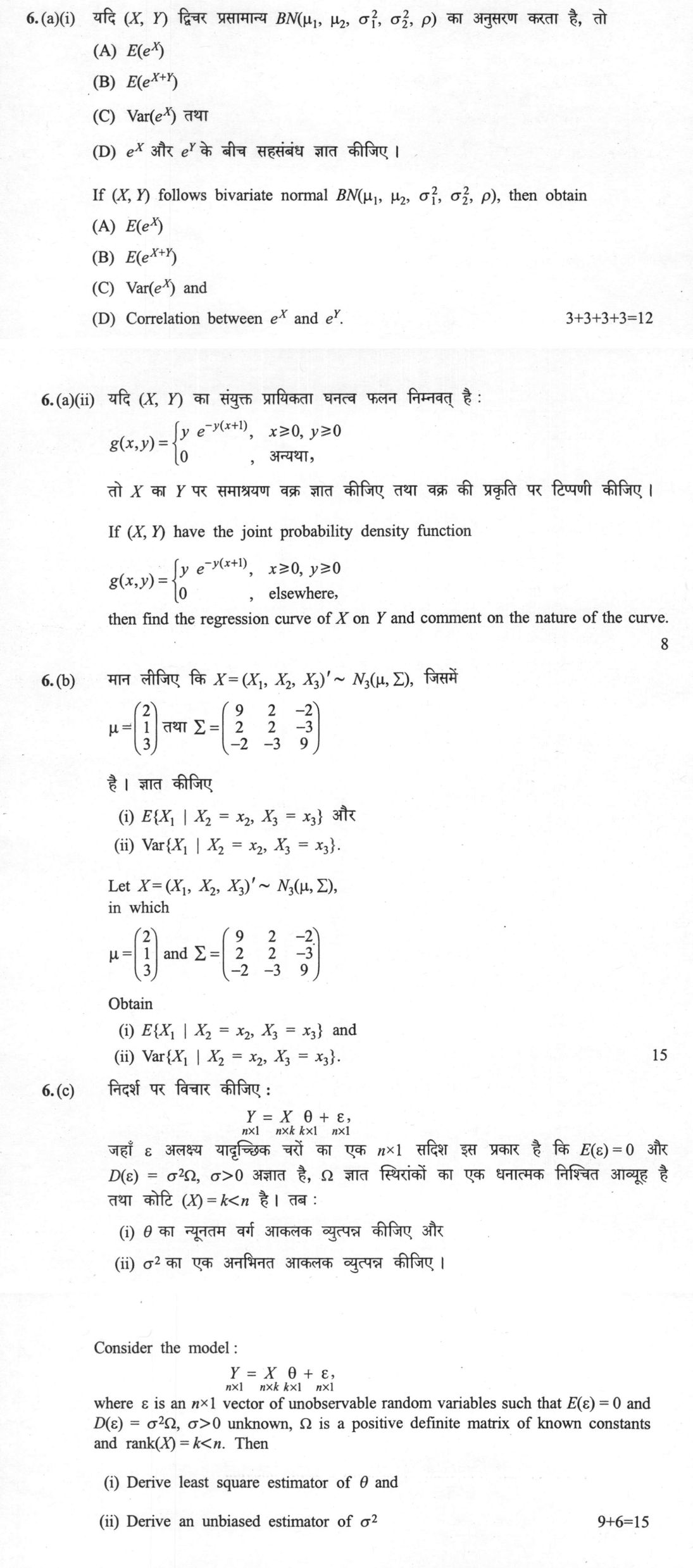
(a)(i) If (X, Y) follows bivariate normal BN(μ₁, μ₂, σ₁², σ₂², ρ), then obtain (A) E(e^X) (B) E(e^(X+Y)) (C) Var(e^X) and (D)…

(a)

(i) Since (X, Y) is bivariate normal, X ~ N(μ₁, σ₁²) and X+Y ~ N(μ₁+μ₂, σ₁²+σ₂²+2ρσ₁σ₂).

The mgf of a normal variable is E(e^(tZ)) = exp(μt + σ²t²/2).

(A) Put Z = X and t = 1: E(e^X) = exp(μ₁ + σ₁²/2).

(B) Put Z = X+Y and t = 1: E(e^(X+Y)) = exp(μ₁+μ₂ + (σ₁²+σ₂²+2ρσ₁σ₂)/2).

(C) Var(e^X) = E(e^(2X)) − (E(e^X))². Now E(e^(2X)) = exp(2μ₁ + 2σ₁²), and (E(e^X))² = exp(2μ₁ + σ₁²). Hence Var(e^X) = exp(2μ₁+σ₁²)(exp(σ₁²)−1).

(D) Cov(e^X, e^Y) = E(e^(X+Y)) − E(e^X)E(e^Y). Since E(e^Y) = exp(μ₂ + σ₂²/2), Cov(e^X, e^Y) = exp(μ₁+μ₂+(σ₁²+σ₂²)/2)(exp(ρσ₁σ₂)−1). Also Var(e^Y) = exp(2μ₂+σ₂²)(exp(σ₂²)−1). Therefore Corr(e^X, e^Y) = (exp(ρσ₁σ₂)−1) / sqrt((exp(σ₁²)−1)(exp(σ₂²)−1)), provided σ₁ > 0 and σ₂ > 0.

(ii) The joint pdf is g(x,y) = y e^(−y(x+1)), x ≥ 0, y ≥ 0.

Marginal of Y: f_Y(y) = ∫₀^∞ y e^(−y(x+1)) dx = y e^(−y) ∫₀^∞ e^(−yx) dx = y e^(−y) · 1/y = e^(−y), y ≥ 0. So Y ~ Exp(1).

Conditional pdf of X given Y = y: f_X|Y(x | y) = g(x,y)/f_Y(y) = y e^(−yx), x ≥ 0. Thus X | Y = y ~ Exp(rate y), whose mean is 1/y. Hence the regression curve of X on Y is E(X | Y = y) = 1/y, y > 0. It is a rectangular hyperbola: nonlinear, decreasing and convex. As y → 0⁺, E(X | Y=y) → ∞; as y → ∞, E(X | Y=y) → 0.

(b)

Partition X₁ and X₂* = (X₂, X₃)′. Here μ₁ = 2, μ₂* = (1, 3)′, Σ₁₁ = 9, Σ₁₂ = [2, −2], Σ₂₂ = [[2, −3], [−3, 9]].

For multivariate normal, E(X₁ | X₂*=x₂*) = μ₁ + Σ₁₂ Σ₂₂⁻¹ (x₂* − μ₂*), Var(X₁ | X₂*=x₂*) = Σ₁₁ − Σ₁₂ Σ₂₂⁻¹ Σ₂₁.

Now det(Σ₂₂) = 2·9 − (−3)(−3) = 9, so Σ₂₂⁻¹ = (1/9) [[9, 3], [3, 2]]. Then Σ₁₂ Σ₂₂⁻¹ = [2, −2] (1/9)[[9, 3], [3, 2]] = [4/3, 2/9]. Hence E(X₁ | X₂=x₂, X₃=x₃) = 2 + (4/3)(x₂−1) + (2/9)(x₃−3). Simplifying, E(X₁ | X₂=x₂, X₃=x₃) = (4/3)x₂ + (2/9)x₃.

Also Σ₁₂ Σ₂₂⁻¹ Σ₂₁ = [4/3, 2/9] [2, −2]′ = 8/3 − 4/9 = 20/9. Therefore Var(X₁ | X₂=x₂, X₃=x₃) = 9 − 20/9 = 61/9.

(c)

The model is Y = Xθ + ε, E(ε)=0, D(ε)=σ²Ω, with Ω positive definite and rank(X)=k<n.

(i) Since Ω is positive definite, write Ω⁻¹ = Ω^(−1/2)Ω^(−1/2). Transform Z = Ω^(−1/2)Y, A = Ω^(−1/2)X, η = Ω^(−1/2)ε. Then Z = Aθ + η, with E(η)=0 and D(η)=σ²I_n. Apply ordinary least squares to the transformed model. Minimize (Z − Aθ)′(Z − Aθ) = (Y − Xθ)′Ω⁻¹(Y − Xθ). The normal equation is A′Aθ = A′Z, i.e. X′Ω⁻¹X θ = X′Ω⁻¹Y. Since rank(X)=k and Ω⁻¹ is positive definite, X′Ω⁻¹X is nonsingular. Hence the generalized least squares estimator is θ̂ = (X′Ω⁻¹X)⁻¹X′Ω⁻¹Y.

(ii) The transformed residual is ê = Z − Aθ̂ = (I − H)η, where H = A(A′A)⁻¹A′ is the projection matrix of rank k. Therefore E(ê′ê) = σ² tr(I − H) = σ²(n − k). But ê′ê = (Y − Xθ̂)′Ω⁻¹(Y − Xθ̂). Thus an unbiased estimator of σ² is σ̂² = (Y − Xθ̂)′Ω⁻¹(Y − Xθ̂)/(n − k). This is valid because n > k and X′Ω⁻¹X is nonsingular.